Introduction
In this example, we check the correctness of SFEMaNS for a thermo-magnetohydrodynamic problem with a rotating force around the vertical axis. This test uses Dirichlet boundary conditions. We note this test does not involve manufactured solutions and consists of checking four quantities, like the \(\bL^2\) norm of the velocity, are the same than the values of reference.
We solve the temperature equation:
\begin{align*} \partial_t T+ \bu \cdot \GRAD T - \kappa \LAP T &= 0, \\ T_{|\Gamma} &= T_\text{bdy} , \\ T_{|t=0} &= T_0, \end{align*}
the Navier-Stokes equations:
\begin{align*} \partial_t\bu+\left(\ROT\bu + 2 \epsilon \textbf{e}_z \right)\CROSS\bu - \frac{1}{\Re}\LAP \bu +\GRAD p &= \alpha T (r\textbf{e}_r+z\textbf{e}_z) + (\ROT \textbf{H}) \times (\mu^c \textbf{H}), \\ \DIV \bu &= 0, \\ \bu_{|\Gamma} &= \bu_{\text{bdy}} , \\ \bu_{|t=0} &= \bu_0, \\ p_{|t=0} &= p_0, \end{align*}
and the Maxwell equations:
\begin{align*} \partial_t (\mu^c \mathbf{H}) + \nabla \times \left(\frac{1}{\Rm \sigma}\nabla \times \mathbf{H} \right) & = \nabla\times (\bu \times \mu^c \mathbf{H}), \\ \text{div} (\mu^c \mathbf {H}) &= 0 ,\\ {\bH \times \bn}_{|\Gamma} &= {\bH_{\text{bdy}} \times \bn}_{|\Gamma},\\ \bH_{|t=0}&= \bH_0. \end{align*}
Theses equations are solved in the domain \(\Omega= \{ (r,\theta,z) \in {R}^3 : (r,\theta,z) \in [0,1] \times [0,2\pi) \times [0,1] \; | \; R_i \leq \sqrt{r^2+z^2} \leq R_o\} \) with \(R_i=7/13\), \(R_o=20/13\) and \(\Gamma= \partial \Omega\). We denote by \(\textbf{e}_r\), respectively \(\textbf{e}_z\), the unit vector in the radial direction, respectively vertical direction. We solve these equation in the mantle frame, meaning we set homogeneous Dirichlet boundary conditions of the velocity field. It explains the presence of the term \( 2 \epsilon \textbf{e}_z \CROSS\bu \) in the Navier-Stokes equations where \(\epsilon\) is the angular velocity. The data are the boundary datas \(T_\text{bdy}, \bu_{\text{bdy}}, \bH_{\text{bdy}}\), the initial data \(T_0, \bu_0, p_0, \bH_0\). The parameters are the thermal diffusivityr \(\kappa\), the kinetic Reynolds number \(\Re\), the thermal gravity number \(\alpha\), the magnetic Reynolds number \(\Rm\), the magnetic permeability \(\mu^c\) and the conductivity \(\sigma\) of the fluid.
Manufactured solutions
As mentionned earlier this test does not involve manufactured solutions. As a consequence, we do not consider specific source term and only initialize the variables to approximate.
The temperature is iniatialized as follows:
\begin{align*} T(r,\theta,z, t=0) & = \frac{R_i R_o}{\sqrt{r^2 + z^2}} - R_i + \frac{21}{\sqrt{12920 \pi}} (1- 3x^2 +3x^4 -x^6)\sin( \varphi)^4 \sin(4\theta) , \end{align*}
where \( x = 2 \sqrt{r^2+z^2} - R_i - R_o \) and \(\varphi=atan2(r,z)\) is the polar angle of the spherical coordinate system.
The initial velocity field and pressure are set to zero.
\begin{align*} u_r(r,\theta,z,t=0) &= 0, \\ u_{\theta}(r,\theta,z,t=0) &= 0, \\ u_z(r,\theta,z,t=0) &= 0, \\ p(r,\theta,z,t=0) &= 0. \end{align*}
The magnetic field is iniatialized as follows:
\begin{align*} \\ H_r(r,\theta,z,t=0) &= 2 \sqrt{10^{-4}} \left( B_1(r,\theta,z) \sin(\varphi) + B_2(r,\theta,z) \cos(\varphi) \right), \\ H_{\theta}(r,\theta,z,t=0) &= 2 \sqrt{10^{-4}} \sin(2\varphi)\frac{15}{8\sqrt{2}} \sin\left(\pi(\sqrt{r^2+z^2} - R_i)\right), \\ H_z(r,\theta,z,t=0) &= 2 \sqrt{10^{-4}}\left( B_1(r,\theta,z) \cos(\varphi) - B_2(r,\theta,z) \sin(\varphi) \right), \end{align*}
where we define \(\varphi\) as previously while \( B_1\) and \(B_2\) are defined as follows:
\begin{align*} B_1(r,\theta,z) &= \cos(\varphi)\frac{5}{8\sqrt{2}} \frac{\left( -48 R_i R_o + (4 R_o + R_i(4+3 R_o)) 6 \sqrt{r^2+z^2} - 4(4+3(R_i+R_o))(r^2+z^2) + 9 (r^2+z^2)^{3/2}\right)}{\sqrt{r^2+z^2}}, \\ B_2(r,\theta,z) &= \sin(\varphi)\frac{-15}{4\sqrt{2}} \frac{(\sqrt{r^2+z^2}-R_i)(\sqrt{r^2+z^2}-R_o)(3\sqrt{r^2+z^2}-4)}{\sqrt{r^2+z^2}}. \end{align*}
The boundary datas \(T_\text{bdy}, \bu_{\text{bdy}}, \bH_{\text{bdy}}\) are computed accordingly.
Generation of the mesh
The finite element mesh used for this test is named Mesh_BENCH1_20.FEM. The mesh size is \(0.05\) for the P1 approximation. You can generate this mesh with the files in the following directory: ($SFEMaNS_MESH_GEN_DIR)/EXAMPLES/EXAMPLES_MANUFACTURED_SOLUTIONS/Mesh_BENCH1_20. The following image show the mesh for P1 finite elements.
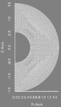
Finite element mesh (P1).
|
Information on the file condlim.f90
The initial conditions, boundary conditions and the forcing terms are set in the file condlim_test_11.f90. Here is a description of the subroutines and functions of interest.
-
First we define the numbers \({test11}_{Ri}\), \({test11}_{Ro}\), \({test11}_{Rossby}\) and \(\pi\) at the begining of the module so that every subroutines has access to these real numbers.
REAL(KIND=8), PRIVATE :: test11_Ri=7/13d0, test11_Ro=20/13d0, test11_Rossby=1.d-4
REAL(KIND=8) :: pi=ACOS(-1.d0)
-
The subroutine
init_velocity_pressure initializes the velocity field and the pressure at the time \(-dt\) and \(0\) with \(dt\) being the time step. It is done by using the functions vv_exact and pp_exact as follows: time = 0.d0
DO i= 1, SIZE(list_mode)
mode = list_mode(i)
DO j = 1, 6
!===velocity
un_m1(:,j,i) = vv_exact(j,mesh_f%rr,mode,time-dt)
un (:,j,i) = vv_exact(j,mesh_f%rr,mode,time)
END DO
DO j = 1, 2
!===pressure
pn_m2(:) = pp_exact(j,mesh_c%rr,mode,time-2*dt)
pn_m1 (:,j,i) = pp_exact(j,mesh_c%rr,mode,time-dt)
pn (:,j,i) = pp_exact(j,mesh_c%rr,mode,time)
phin_m1(:,j,i) = pn_m1(:,j,i) - pn_m2(:)
phin (:,j,i) = Pn (:,j,i) - pn_m1(:,j,i)
ENDDO
ENDDO
-
The subroutine
init_temperature initializes the temperature at the time \(-dt\) and \(0\) with \(dt\) being the time step. It is done by using the function temperature_exact as follows: time = 0.d0
DO i= 1, SIZE(list_mode)
mode = list_mode(i)
DO j = 1, 2
tempn_m1(:,j,i) = temperature_exact(j, mesh%rr, mode, time-dt)
tempn (:,j,i) = temperature_exact(j, mesh%rr, mode, time)
ENDDO
ENDDO
-
The function
vv_exact contains the analytical velocity field. It is used to initialize the velocity field and to impose Dirichlet boundary conditions on the velocity field. It is set to zero.
-
The function
pp_exact contains the analytical pressure. It is used to initialize the pressure and is set to zero.
-
The function
temperature_exact contains the analytical temperature. It is used to initialize the temperature and to impose Dirichlet boundary condition on the temperature.
-
We construct the radial and vertical coordinates r, z.
-
For the Fourier modes \(m\in \{0,4\}\) we define the temperature depending of its TYPE (1 for cosine and 2 for sine) as follows:
IF (m==0 .OR. m==4) THEN
DO n = 1, SIZE(rr,2)
rho(n)=SQRT(rr(1,n)**2+rr(2,n)**2)
theta=ATAN2(rr(1,n),rr(2,n))
x=2*rho(n) - test11_Ri - test11_Ro
A(n)=(21/SQRT(17920*Pi))*(1-3*x**2+3*x**4-x**6)*SIN(
theta)**4
END DO
IF (m==0 .AND. TYPE==1) THEN
vv=( test11_Ri*test11_Ro/rho)- test11_Ri
ELSE IF (m==4 .AND. TYPE==1) THEN
vv= A
ELSE
vv = 0.d0
END IF
-
For the other Fourier modes, we set the temperature to zero.
ELSE
vv = 0.d0
END IF
RETURN
-
The function
source_in_temperature computes the source term, denoted \(f_T\) in previous tests, of the temperature equation. As it is not used in this test, we set it to zero.
-
The function
source_in_NS_momentum computes the source term \(\alpha T(r\textbf{e}_r+z\textbf{e}_z) \) of the Navier-Stokes equations.
-
We construct the radial and vertical coordinates r, z.
-
We compute the term \(\alpha T r\textbf{e}_r\) (component radial so TYPE 1 and 2).
IF (TYPE==1) THEN
vv = inputs%gravity_coefficient*opt_tempn(:,1,i)*r
ELSE IF (TYPE==2) THEN
vv = inputs%gravity_coefficient*opt_tempn(:,2,i)*r
-
We compute the term \(\alpha T z\textbf{e}_z\) (component vertical so TYPE 5 and 6).
ELSE IF (TYPE==5) THEN
vv = inputs%gravity_coefficient*opt_tempn(:,1,i)*
zELSE IF (TYPE==6) THEN
vv = inputs%gravity_coefficient*opt_tempn(:,2,i)*
z
-
The azimuthal component of this source term is set to zero.
ELSE
vv = 0.d0
END IF
RETURN
-
The subroutine
init_maxwell initializes the magnetic field at the time \(-dt\) and \(0\) with \(dt\) being the time step. We remind the initial magnetic field only depends of the Fourier mode \(m=0\). Firslty we define it for spherical coordinates (Brho, Btheta, Bphi) so we can later define for cylindrical coordinates depending of its TYPE (1 and 2 for the component radial cosine and sine, 3 and 4 for the component azimuthal cosine and sine, 5 and 6 for the component vertical cosine and sine). Hn = 0.d0
DO i = 1, SIZE(list_mode)
IF (list_mode(i) /= 0) CYCLE
normalization = 2*SQRT(test11_Rossby)
DO n=1,SIZE(H_mesh%rr,2)
rho = SQRT(H_mesh%rr(1,n)**2+H_mesh%rr(2,n)**2)
theta(n) = ATAN2(H_mesh%rr(1,n),H_mesh%rr(2,n))
Brho(n) = COS(
theta(n))*5.d0/(SQRT(2d0)*8d0)*(-48d0*test11_Ri*test11_Ro &
+ (4*test11_Ro+test11_Ri*(4+3*test11_Ro))*6*rho &
-4*(4+3*(test11_Ri+test11_Ro))*rho**2+9*rho**3)/rho
Btheta(n)= SIN(
theta(n))*(-15d0/(SQRT(2d0)*4d0))*((rho-test11_Ri)*(rho-test11_Ro)*(3*rho-4))/rho
Bphi(n) = SIN(2*
theta(n))*(15d0/(SQRT(2d0)*8d0))*SIN(Pi*(rho-test11_Ri))
END DO
Hn(:,1,i) = normalization*(Brho*SIN(
theta) + Btheta*COS(
theta))
Hn(:,3,i) = normalization*Bphi
Hn(:,5,i) = normalization*(Brho*COS(
theta) - Btheta*SIN(
theta))
END DO
Hn1 = Hn
time = 0.d0
phin =0.d0
phin1=0.d0
RETURN
-
The function
Hexact contains the analytical magnetic field. It is used to impose Dirichlet boundary conditions on \(\textbf{H}\times\textbf{n}\) with \(\textbf{n}\) the outter normal vector.
-
The function
Jexact_gauss is used to define the source term \(\textbf{j}\) that is not used in this test. So we set it to zero.
All the other subroutines present in the file condlim_test_11.f90 are not used in this test. We refer to the section Fortran file condlim.f90 for a description of all the subroutines of the condlim file.
Setting in the data file
We describe the data file of this test. It is called debug_data_test_11 and can be found in the following directory: ($SFEMaNS_DIR)/MHD_DATA_TEST_CONV_PETSC.
-
We use a formatted mesh by setting:
===Is mesh file formatted (true/false)?
.t.
-
The path and the name of the mesh are specified with the two following lines:
===Directory and name of mesh file
'.' 'Mesh_BENCH1_20.FEM'
-
We use two processors in the meridian section. It means the finite element mesh is subdivised in two. To do so, we write:
===Number of processors in meridian section
2
-
We solve the problem for \(3\) Fourier modes.
===Number of Fourier modes
3
-
We use \(3\) processors in Fourier.
===Number of processors in Fourier space
3
-
We select specific Fourier modes to solve.
===Select Fourier modes? (true/false)
-
We give the list of the Fourier modes to solve.
===List of Fourier modes (if select_mode=.TRUE.)
0 4 8
-
We approximate the Maxwell and the Navier-Stokes equations by setting:
===Problem type: (nst, mxw, mhd, fhd)
'mhd'
-
We do not restart the computations from previous results.
===Restart on velocity (true/false)
.f.
===Restart on magnetic field (true/false)
.f.
-
We use a time step of \(0.02\) and solve the problem over \(20\) time iterations.
===Time step and number of time iterations
2d-2, 20
-
We set the number of domains and their label, see the files associated to the generation of the mesh, where the code approximates the Navier-Stokes equations,
===Number of subdomains in Navier-Stokes mesh
1
===List of subdomains for Navier-Stokes mesh
1
-
We set the number of boundaries with Dirichlet conditions on the velocity field and give their respective labels.
===How many
boundary pieces
for full Dirichlet BCs on velocity?
2
===List of
boundary pieces
for full Dirichlet BCs on velocity
2 4
-
We set the kinetic Reynolds number \(\Re\).
===Reynolds number
1000d0
-
We want to take into account a rotating force of axis \(\textbf{e}_z\) and angular velocity \(\epsilon\) in the wall frame. So we add the term \( 2\epsilon \textbf{e}_z \times \bu \) in the left hand side of the Navier-Stokes equations. Such features is already programmed in SFEMaNS via the following lines in your data file.
-
We set the option precession to true.
===Is there a precession term (true/false)?
.t.
-
We set the precession rate \(\epsilon\) and the precesion angle \(\alpha\).
===Precession rate
1.d0
===Precession angle over pi
0.d0
-
We give information on how to solve the matrix associated to the time marching of the velocity.
-
===Maximum number of iterations for velocity solver
100
-
===Relative tolerance for velocity solver
1.d-6
===Absolute tolerance for velocity solver
1.d-10
-
===Solver type for velocity (FGMRES, CG, ...)
GMRES
===Preconditionner type for velocity solver (HYPRE, JACOBI, MUMPS...)
MUMPS
-
We give information on how to solve the matrix associated to the time marching of the pressure.
-
===Maximum number of iterations for pressure solver
100
-
===Relative tolerance for pressure solver
1.d-6
===Absolute tolerance for pressure solver
1.d-10
-
===Solver type for pressure (FGMRES, CG, ...)
GMRES
===Preconditionner type for pressure solver (HYPRE, JACOBI, MUMPS...)
MUMPS
-
We give information on how to solve the mass matrix.
-
===Maximum number of iterations for mass matrix solver
100
-
===Relative tolerance for mass matrix solver
1.d-6
===Absolute tolerance for mass matrix solver
1.d-10
-
===Solver type for mass matrix (FGMRES, CG, ...)
CG
===Preconditionner type for mass matrix solver (HYPRE, JACOBI, MUMPS...)
MUMPS
-
We solve the temperature equation (in the same domain than the Navier-Stokes equations).
===Is there a temperature field?
.t.
-
We set the number of domains and their label, see the files associated to the generation of the mesh, where the code approximated the temperature equation.
===Number of subdomains in temperature mesh
1
===List of subdomains for temperature mesh
1
-
We set the thermal diffusivity \(\kappa\).
===Diffusivity coefficient for temperature
1.d-3
-
We set the thermal gravity number \(\alpha\).
===Non-dimensional gravity coefficient
0.065
-
We set the number of boundaries with Dirichlet conditions on the temperature and give their respective labels.
===How many
boundary pieces
for Dirichlet BCs on temperature?
2
===List of
boundary pieces
for Dirichlet BCs on temperature
2 4
-
We give information on how to solve the matrix associated to the time marching of the temperature.
-
===Maximum number of iterations for temperature solver
100
-
===Relative tolerance for temperature solver
1.d-6
===Absolute tolerance for temperature solver
1.d-10
-
===Solver type for temperature (FGMRES, CG, ...)
GMRES
===Preconditionner type for temperature solver (HYPRE, JACOBI, MUMPS...)
MUMPS
-
We set the number of domains and their label, see the files associated to the generation of the mesh, where the code approximates the magnetic field.
===Number of subdomains in magnetic field (H) mesh
1
===List of subdomains for magnetic field (H) mesh
1
-
We set the number of interface in H_mesh.
===Number of interfaces in H mesh
0
-
We set the number of boundaries with Dirichlet conditions on the magnetic field and give their respective labels.
===Number of Dirichlet sides for Hxn
2
===List of Dirichlet sides for Hxn
2 4
-
We set the magnetic permeability in each domains where the magnetic field is approximated.
===Permeability in the conductive part (1:nb_dom_H)
1.d0
-
We set the conductivity in each domains where the magnetic field is approximated.
===Conductivity in the conductive part (1:nb_dom_H)
1.d0
-
We set the type of finite element used to approximate the magnetic field.
===Type of finite element for magnetic field
2
-
We set the magnetic Reynolds number \(\Rm\).
===Magnetic Reynolds number
5000d0
-
We set stabilization coefficient for the divergence of the magnetic field and the penalty of the Dirichlet and interface terms.
===Stabilization coefficient (divergence)
1.d0
===Stabilization coefficient for Dirichlet H and/or interface H/H
100.d0
-
We set the number of domains and their label, see the files associated to the generation of the mesh, where the code approximates the scalar potential.
===Number of subdomains in magnetic potential (phi) mesh
0
-
We give information on how to solve the matrix associated to the time marching of the Maxwell equations.
-
===Maximum number of iterations for Maxwell solver
100
-
===Relative tolerance for Maxwell solver
1.d-6
===Absolute tolerance for Maxwell solver
1.d-10
-
===Solver type for Maxwell (FGMRES, CG, ...)
GMRES
===Preconditionner type for Maxwell solver (HYPRE, JACOBI, MUMPS...)
MUMPS
Outputs and value of reference
The outputs of this test are computed with the file post_processing_debug.f90 that can be found in the following directory: ($SFEMaNS_DIR)/MHD_DATA_TEST_CONV_PETSC.
To check the well behavior of the code, we compute four quantities:
-
The H1 norm of the velocity.
-
The L2 norm of the magnetic field.
-
The L2 norm of the pressure.
-
The L2 norm of the temperature
These quantities are computed at the final time \(t=0.4\). They are compared to reference values to attest of the correctness of the code. These values of reference are in the last lines of the file debug_data_test_11 in the directory ($SFEMaNS_DIR)/MHD_DATA_TEST_CONV_PETSC. They are equal to:
============================================
Mesh_BENCH1_20.FEM, P2
===Reference results
0.14529939453854082 H1 norm of velocity
0.16031055031353644 L2 norm of magnetic field
1.47953318917485640E-002 L2 norm of pressure
1.1061039638796786 L2 norm of temperature
To conclude this test, we show the profile of the approximated pressure, velocity magnitude, temperature and magnetic field magnitude at the final time. These figures are done in the plane \(y=0\) which is the union of the half plane \(\theta=0\) and \(\theta=\pi\).
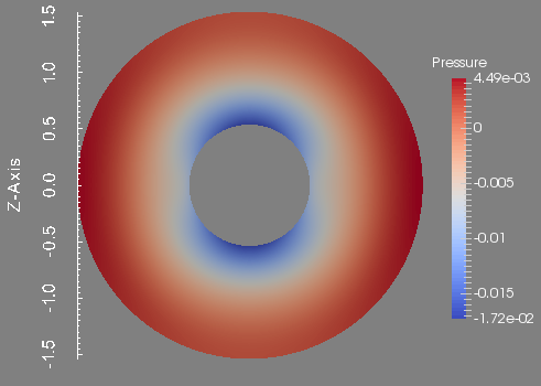
Pressure in the plane plane y=0.
|
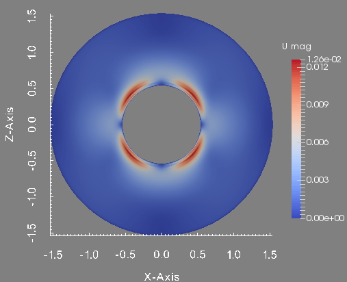
Velocity magnitude in the plane plane y=0.
|
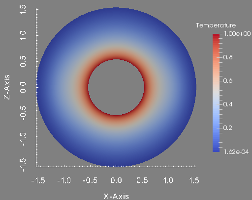
Temperature in the plane plane y=0.
|
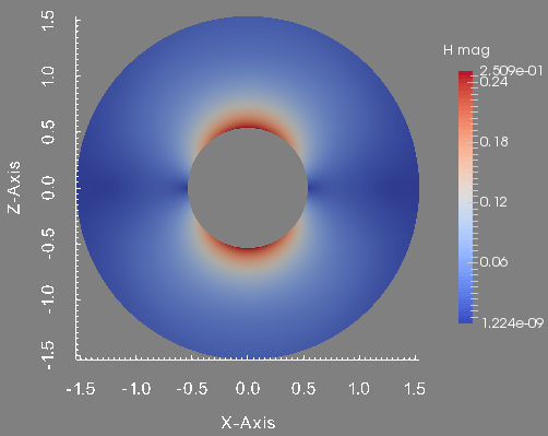
Magnetic field magnitude in the plane plane y=0.
|
 1.8.5
1.8.5 
