Introduction
In this example, we check the correctness of SFEMaNS for stationary magnetic problem involving a conducting. The magnetic permeability is variable in z and presents a smooth jump. The magnetic permeability is given. We consider Dirichlet boundary conditions. We use P2 finite elements. This set up is approximated over one time iteration with a large time step.
We solve the Maxwell equations with the magnetic field \(\bB=\mu \bH\) as dependent variable:
\begin{align} \begin{cases} \partial_t (\mathbf{B}) + \nabla \times \left(\frac{1}{\Rm \sigma}\nabla \times( \frac{1}{\mu^c}\mathbf{B} ) \right) = \nabla\times (\bu^\text{given} \times \mathbf{B}) + \nabla \times \left(\frac{1}{\Rm \sigma} \nabla\times \mathbf{j} \right) & \text{in } \Omega, \\ \text{div} (\mathbf{B}) = 0 & \text{in } \Omega ,\\ {\bH \times \bn}_{|\Gamma} = {\bH_{\text{bdy}} \times \bn}_{|\Gamma}, &\\ \bH_{|t=0}= \bH_0, \\ \end{cases} \end{align}
in the domain \(\Omega= \{ (r,\theta,z) \in {R}^3 : (r,\theta,z) \in [0,0.5] \times [0,2\pi) \times [-0.2,0.2]\} \). We set \(\Gamma= \partial \Omega\). We also define the outward normal \(\bn\) to the surface \(\Gamma\). The data are the source term \(\mathbf{j}\), the given velocity \(\bu^\text{given}\), the boundary data \(\bH_{\text{bdy}}\) and the initial data \(\bH_0\). The parameter \(\Rm\) is the magnetic Reynolds number. The parameter \(\mu^c\) is the magnetic permeability of the conducting region \(\Omega\). The parameter \(\sigma\) is the conductivity in the conducting region \(\Omega\).
Manufactured solutions
We define the magnetic permeability in the conducting region as follows:
\begin{align*} \mu^c(z)= \begin{cases} \mu_{26}& \text{ for } z\leq z_1, \\ 1+ (\mu_{26}-1)F_z(z) &\text{ for } z_1 \leq z \leq z_0, \\ 1 &\text{ for } z_0 \leq z, \end{cases} \end{align*}
where \(\mu_{26}=5\), \(z_0=0\), \(z_1=-0.032\) and \(F_z\) is the polynomial function of order 2 such that \(F_z(z_0)=0\), \(F_z(z_1)=1\) and \(\partial_z F_z(\frac{z_0+z_1}{2})=0\).
We approximate the following analytical solutions:
\begin{align*} H_r(r,\theta,z,t) &= \frac{\alpha_{26}m_{26} r^{m_{26}-1}}{\mu^c(z)}\cos(m_{26}\theta), \\ H_{\theta}(r,\theta,z,t) &=-\frac{\alpha_{26}m_{26} r^{m_{26}-1}}{\mu^c(z)}\sin(m_{26}\theta), \\ H_z(r,\theta,z,t) &= 0, \end{align*}
with \(\alpha_{26}=1\) and \(m_{26}=4\). We also remind that \(\bB=\mu\bH\).
We also set the given velocity field to zero.
\begin{align*} u^\text{given}_r(r,\theta,z,t) &= 0, \\ u^\text{given}_{\theta}(r,\theta,z,t) &= 0, \\ u^\text{given}_z(r,\theta,z,t) &= 0. \end{align*}
The source term \( \mathbf{j}\) and the boundary data \(\bH_{\text{bdy}}\) are computed accordingly.
Generation of the mesh
The finite element mesh used for this test is named mesh_26_0.03.FEM. The mesh size for the P1 approximation is \(0.03\) in \(\Omega\). You can generate this mesh with the files in the following directory: ($SFEMaNS_MESH_GEN_DIR)/EXAMPLES/EXAMPLES_MANUFACTURED_SOLUTIONS/mesh_26_0.03.FEM. The following images show the mesh for P1 finite elements for the conducting and vacuum regions.
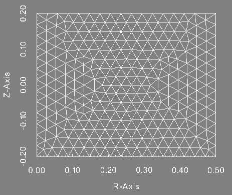
Finite element mesh (P1) of the conducting region.
|
Information on the file condlim.f90
The initial conditions, boundary conditions and the forcing term \(\textbf{j}\) in the Maxwell equations are set in the file condlim_test_26.f90. This condlim also uses functions of the file test_26.f90 to define the magnetic permeability and its gradient. Here is a description of the subroutines and functions of interest of the file condlim_test_26.f90.
-
The subroutine
init_maxwell initializes the magnetic field at the time \(-dt\) and \(0\) with \(dt\) being the time step. It is set to zero. Hn1 = 0.d0
Hn = 0.d0
phin1 = 0.d0
phin = 0.d0
time =0.d0
RETURN
-
The function
Hexact contains the analytical magnetic field. It is used to impose Dirichlet boundary conditions on \(\textbf{H}\times\textbf{n}\) with \(\textbf{n}\) the outter normal vector.
-
If the Fourier mode m is not equal to \(m_{26}\), we set the magnetic field to zero.
vv = 0.d0
IF (m .NE. test_mode_T26 ) THEN
RETURN
ENDIF
-
We define the radial and vertical coordinates \((r, z)\).
-
For the Fourier mode \(m=m_{26}\), we define the magnetic field depending of its TYPE (1 and 2 for the component radial cosine and sine, 3 and 4 for the component azimuthal cosine and sine, 5 and 6 for the component vertical cosine and sine) as follows:
DO n = 1, SIZE(rr,2)
tmp= alpha_T26*test_mode_T26*r(n)**(test_mode_T26-1)/mu_func_T26(r(n),
z(n))
IF (type==1) THEN
vv(n) = tmp
ELSE IF (type==4) THEN
vv(n) = -tmp
ENDIF
END DO
RETURN
test_26.f90. The function mu_func_T26 is also defined in the file test_26.f90, it is equal to the magnetic permeability.
-
The function
Vexact is used to define the given velocity field \(\bu^\text{given}\). It is set to zero.
-
The function
Jexact_gauss is used to define the source term \(\textbf{j}\). We remind that \( \bu^\text{given}=0 \) and \(\partial_t \textbf{H}=0\) so it is defined such that \(\textbf{j}=\ROT \bH\).
-
If the Fourier mode m is not equal to \(m_{26}\), we set the \(\textbf{j}\) to zero.
vv = 0.d0
IF (m .NE. test_mode_T26) THEN
RETURN
ENDIF
-
We define the radial and vertical coordinates \((r,z)\).
-
We define the z-derivative of the magnetic permeability (only depends of z) with the function
Dmu_func_T26 defined in the file test_26.f90.
-
For the Fourier mode \(m=m_{26}\), we define the source term depending of its TYPE (1 and 2 for the component radial cosine and sine, 3 and 4 for the component azimuthal cosine and sine, 5 and 6 for the component vertical cosine and sine) as follows:
tmp=alpha_T26*test_mode_T26*r**(test_mode_T26-1)*(-1.d0/mu_func_T26(r,
z)**2)
IF (type==2) THEN
vv = tmp*Dmu(2)
ELSE IF (type==3) THEN
vv = tmp*Dmu(2)
ELSE IF (type==6) THEN
vv = - tmp*Dmu(1)
ENDIF
RETURN
-
The function
mu_bar_in_fourier_space defines the magnetic permeability that depends of the radial and vertical coordinates. It is done by using the function mu_bar_in_fourier_space_anal_T26 of the file test_26.f90. IF( PRESENT(pts) .AND. PRESENT(pts_ids) ) THEN
vv=mu_bar_in_fourier_space_anal_T26(H_mesh,nb,ne,pts,pts_ids)
ELSE
vv=mu_bar_in_fourier_space_anal_T26(H_mesh,nb,ne,pts)
END IF
RETURN
mu_in_real_space.
-
The function
grad_mu_bar_in_fourier_space defines the gradient of the magnetic permeability. It is done by using the function grad_mu_bar_in_fourier_space_anal_T26 of the file test_26.f90. vv=grad_mu_bar_in_fourier_space_anal_T26(pt,pt_id)
RETURN
All the other subroutines present in the file condlim_test_26.f90 are not used in this test. We refer to the section Fortran file condlim.f90 for a description of all the subroutines of the condlim file. The following describes the functions of interest of the file test_26.f90.
-
First we define the real numbers \(\mu_{26}\), \(\alpha_{26}\) and the integer \(m_{26}\).
REAL(KIND=8), PARAMETER:: mu_disk_T26 = 5.d0
REAL(KIND=8), PARAMETER:: alpha_T26 = 1.d0
INTEGER, PARAMETER :: test_mode_T26 = 4;
-
We also define the vertical coordinates \(z_0\) and \(z_1\) (denoted zm_T26 and z1_T26).
REAL(KIND=8), PARAMETER:: wjump_T26 = 0.032d0*(1.0d0)
REAL(KIND=8), PARAMETER:: zm_T26 = 0.d0, z1_T26 = zm_T26-wjump_T26
-
The function
smooth_jump_down_T26 depends of the variable x and is defined such that it is equal to 1 for x= x0 and 0 for x=x1. Moreover its derivative in \(x=\frac{x0+x1}{2}\) is zero. a0 = x1**2*(3*x0-x1)/(x0-x1)**3;
a1 = -6.0*x0*x1/(x0-x1)**3;
a2 = (3.0*(x0+x1))/(x0-x1)**3;
a3 = -2.0/(x0-x1)**3;
vv = a0+a1*x+a2*x*x + a3*x*x*x
RETURN
-
The function
Dsmooth_jump_down_T26 is the derivative of the function smooth_jump_down_T26. a0 = x1**2*(3*x0-x1)/(x0-x1)**3;
a1 = -6.0*x0*x1/(x0-x1)**3;
a2 = (3.0*(x0+x1))/(x0-x1)**3;
a3 = -2.0/(x0-x1)**3;
vv = a1+2.d0*a2*x + 3.d0*a3*x*x
RETURN
-
The function
smooth_jump_up_T26 depends of the variable x and is defined such that it is equal to 1 for x= x1 and 0 for x=x0. Moreover its derivative in \(x=\frac{x0+x1}{2}\) is zero. vv = 1.d0 - smooth_jump_down_T26( x,x0,x1 );
RETURN
-
The function
Dsmooth_jump_up_T26 is the derivative of the function smooth_jump_up_T26. vv = - Dsmooth_jump_down_T26( x,x0,x1 );
RETURN
-
The function
mu_func_T26 is used to defined the magnetic permeability. Fz=smooth_jump_up_T26(
z,zm_T26,z1_T26)
vv = 1.d0
ELSE IF (
z.LE. z1_T26 ) THEN
vv = mu_disk_T26
ELSE
vv = Fz*(mu_disk_T26-1.d0) + 1.d0
END IF
RETURN
-
The function
Dmu_func_T26 is the gradient of the function mu_func_T26. DFz=Dsmooth_jump_up_T26(
z,zm_T26,z1_T26)
vv = 0.d0
ELSE IF (
z.LE. z1_T26 ) THEN
vv = 0.d0
ELSE
vv(1) = 0
vv(2) = DFz*(mu_disk_T26-1.d0)
END IF
RETURN
-
The function
mu_bar_in_fourier_space_anal_T26 defines the magnetic permeability.
-
First we define the radial and vertical cylindrical coordinates of each nodes considered.
IF( PRESENT(pts) .AND. PRESENT(pts_ids) ) THEN !Computing mu at pts
r=pts(1,nb:ne)
ELSE
r=H_mesh%rr(1,nb:ne) !Computing mu at nodes
END IF
-
We define the magnetic permeability on the nodes considered.
DO n = 1, ne - nb + 1
vv(n) = mu_func_T26(r(n),
z(n))
END DO
RETURN
-
The function
grad_mu_bar_in_fourier_space_anal_T18 defines the gradient of the magnetic permeability on gauss points.
-
We define the radial and vertical cylindrical coordinates.
-
We define the gradient of the magnetic permeability.
vv(1)=tmp(1)
vv(2)=tmp(2)
Setting in the data file
We describe the data file of this test. It is called debug_data_test_18 and can be found in the following directory: ($SFEMaNS_DIR)/MHD_DATA_TEST_CONV_PETSC.
-
We use a formatted mesh by setting:
===Is mesh file formatted (true/false)?
.t.
-
The path and the name of the mesh are specified with the two following lines:
===Directory and name of mesh file
'.' 'mesh_26_0.03.FEM'
-
We use one processor in the meridian section. It means the finite element mesh is not subdivised.
===Number of processors in meridian section
1
-
We solve the problem for \(1\) Fourier modes.
===Number of Fourier modes
1
-
We use \(1\) processors in Fourier space.
===Number of processors in Fourier space
1
-
We select specific Fourier modes to solve.
===Select Fourier modes? (true/false)
.t.
-
We give the list of the Fourier modes to solve.
===List of Fourier modes (if select_mode=.TRUE.)
4
-
We approximate the Maxwell equations by setting:
===Problem type: (nst, mxw, mhd, fhd)
'mxw'
-
We do not restart the computations from previous results.
===Restart on velocity (true/false)
.f.
===Restart on magnetic field (true/false)
.f.
-
We use a time step of \(10^{40}\) and solve the problem over \(1\) time iteration.
===Time step and number of time iterations
1.d40 1
-
We use the magnetic field \(\textbf{B}\) as dependent variable for the Maxwell equations.
===Solve Maxwell with H (true) or B (false)?
-
We set the number of domains and their label, see the files associated to the generation of the mesh, where the code approximates the Maxwell equations.
===Number of subdomains in magnetic field (H) mesh
1
===List of subdomains for magnetic field (H) mesh
1
-
We set the number of interface in H_mesh.
===Number of interfaces in H mesh
0
-
We set the number of boundaries with Dirichlet conditions on the magnetic field and give their respective labels.
===Number of Dirichlet sides for Hxn
3
===List of Dirichlet sides for Hxn
4 2 3
-
The magnetic permeability is defined with a function of the file
condlim_test_18.f90. ===Is permeability defined analytically (true/false)?
.t.
-
We construct the magnetic permeability on the gauss points without using its value on the nodes and a finite element interpolation.
===Use FEM Interpolation for magnetic permeability (true/false)?
.f.
-
We set the conductivity in each domains where the magnetic field is approximated.
===Conductivity in the conductive part (1:nb_dom_H)
1.d0
-
We set the type of finite element used to approximate the magnetic field.
===Type of finite element for magnetic field
2
-
We set the magnetic Reynolds number \(\Rm\).
===Magnetic Reynolds number
1.d0
-
We set stabilization coefficient for the divergence of the magnetic field and the penalty of the Dirichlet and interface terms.
===Stabilization coefficient (divergence)
1.d0
===Stabilization coefficient for Dirichlet H and/or interface H/H
1.d0
-
We give information on how to solve the matrix associated to the time marching of the Maxwell equations.
-
===Maximum number of iterations for Maxwell solver
100
-
===Relative tolerance for Maxwell solver
1.d-6
===Absolute tolerance for Maxwell solver
1.d-10
-
===Solver type for Maxwell (FGMRES, CG, ...)
GMRES
===Preconditionner type for Maxwell solver (HYPRE, JACOBI, MUMPS...)
MUMPS
Outputs and value of reference
The outputs of this test are computed with the file post_processing_debug.f90 that can be found in the following directory: ($SFEMaNS_DIR)/MHD_DATA_TEST_CONV_PETSC.
To check the well behavior of the code, we compute four quantities:
-
The L2 norm of the error on the divergence of the magnetic field \(\textbf{B}=\mu\textbf{H}\).
-
The L2 norm of the error on the curl of the magnetic field \(\textbf{H}\).
-
The L2 norm of the error on the magnetic field \(\textbf{H}\).
-
The L2 norm of the magnetic filed \(\bH\).
They are compared to reference values to attest of the correctness of the code. These values of reference are in the last lines of the file debug_data_test_26 in the directory ($SFEMaNS_DIR)/MHD_DATA_TEST_CONV_PETSC. They are equal to:
============================================
mesh_26_0.03.FEM, dt=1.0d40, it_max=1
===Reference results
6.232118631975291E-003 !L2 norm of div(mu (H-Hexact))
1.402063664918604E-003 !L2 norm of curl(H-Hexact)
5.555512428427833E-005 !L2 norm of H-Hexact
0.102653049435891 !L2 norm of H
To conclude this test, we show the profile of the approximated magnetic field \(\textbf{H}\) at the final time. These figures are done in the plane \(y=0\) which is the union of the half plane \(\theta=0\) and \(\theta=\pi\).
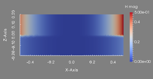
Magnetic field magnitude in the plane plane y=0.
|
 1.8.5
1.8.5 
