Introduction
In this example, we check the correctness of SFEMaNS for a thermohydrodynamic problem involving periodic and Dirichlet boundary conditions.
We solve the temperature equation:
\begin{align*} \partial_t T+ \bu \cdot \GRAD T - \kappa \LAP T &= f_T, \\ T_{|\{z=0\}} &= T_{|\{z=1\}} , \\ T_{|\Gamma} &= T_\text{bdy} , \\ T_{|t=0} &= T_0, \end{align*}
and the Navier-Stokes equations:
\begin{align*} \partial_t\bu+\left(\ROT\bu\right)\CROSS\bu - \frac{1}{\Re}\LAP \bu +\GRAD p &= \alpha T \textbf{e}_z + \bef, \\ \bu_{|\{z=0\}} &= \bu_{|\{z=0.5\}} , \\ p_{|\{z=0\}} &= p_{|\{z=1\}} , \\ \\ \DIV \bu &= 0, \\ \bu_{|\Gamma} &= \bu_{\text{bdy}} , \\ \bu_{|t=0} &= \bu_0, \\ p_{|t=0} &= p_0, \end{align*}
in the domain \(\Omega= \{ (r,\theta,z) \in {R}^3 : (r,\theta,z) \in [0,1/2] \times [0,2\pi) \times [0,1]\} \) with \(\Gamma= \partial \Omega\setminus\{ \{z=0\} \cup \{z=1\} \} \). We denote by \(\textbf{e}_z\) the unit vector in the vertical direction. The data are the source terms \(f_T\) and \(\bef\), the boundary datas \(T_\text{bdy}\) and \(\bu_{\text{bdy}}\), the initial data \(T_0\), \(\bu_0\) and \(p_0\). The parameters are the thermal diffusivity \(\kappa\), the kinetic Reynolds number \(\Re\) and a thermal gravity number \(\alpha\). We remind that these parameters are dimensionless.
Manufactured solutions
We approximate the following analytical solutions:
\begin{align*} T(r,\theta,z,t) & = \left(r^2\sin(2\pi z) + r^2\cos(2\pi z)(\cos(\theta)+2\sin(2\theta))\right)\cos(t), \\ u_r(r,\theta,z,t) &= r^3 \cos(2\pi z)\sin(t), \\ u_{\theta}(r,\theta,z,t) &= r^2 \sin(2\pi z) \sin(t), \\ u_z(r,\theta,z,t) &= -\frac{2r^2}{\pi}\sin(2\pi z) \sin(t), \\ p(r,\theta,z,t) &= \frac{1}{2} \left( r^6\cos(2\pi z)^2 + r^4 \sin(2\pi z)^2 + \frac{4r^4}{\pi^2}\sin(2\pi z)^2 \right) \sin(t)^2, \end{align*}
where the source terms \(f_T, \bef\) and the boundary datas \(T_\text{bdy}, \bu_{\text{bdy}}\) are computed accordingly.
Generation of the mesh
The finite element mesh used for this test is named Mesh_10_form.FEM and has a mesh size of \(0.1\) for the P1 approximation. You can generate this mesh with the files in the following directory: ($SFEMaNS_MESH_GEN_DIR)/EXAMPLES/EXAMPLES_MANUFACTURED_SOLUTIONS/Mesh_10_form. The following image shows the mesh for P1 finite elements.
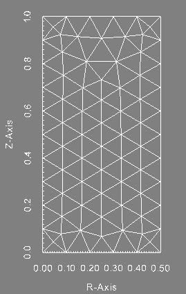
Finite element mesh (P1).
|
Information on the file condlim.f90
The initial conditions, boundary conditions and the forcing terms \(\textbf{f}\) in the Navier-Stokes equations and \(f_T\) in the temperature equation are set in the file condlim_test_9.f90. Here is a description of the subroutines and functions of interest.
-
First we define the number \(\pi\) at the begining of the module so that every subroutines has access to this real number.
REAL(KIND=8) :: pi=ACOS(-1.d0)
-
The subroutine
init_velocity_pressure initializes the velocity field and the pressure at the time \(-dt\) and \(0\) with \(dt\) being the time step. This is done by using the functions vv_exact and pp_exact as follows: time = 0.d0
DO i= 1, SIZE(list_mode)
mode = list_mode(i)
DO j = 1, 6
!===velocity
un_m1(:,j,i) = vv_exact(j,mesh_f%rr,mode,time-dt)
un (:,j,i) = vv_exact(j,mesh_f%rr,mode,time)
END DO
DO j = 1, 2
!===pressure
pn_m2(:) = pp_exact(j,mesh_c%rr,mode,time-2*dt)
pn_m1 (:,j,i) = pp_exact(j,mesh_c%rr,mode,time-dt)
pn (:,j,i) = pp_exact(j,mesh_c%rr,mode,time)
phin_m1(:,j,i) = pn_m1(:,j,i) - pn_m2(:)
phin (:,j,i) = Pn (:,j,i) - pn_m1(:,j,i)
ENDDO
ENDDO
-
The subroutine
init_temperature initializes the temperature at the time \(-dt\) and \(0\) with \(dt\) being the time step. It is done by using the function temperature_exact as follows: time = 0.d0
DO i= 1, SIZE(list_mode)
mode = list_mode(i)
DO j = 1, 2
tempn_m1(:,j,i) = temperature_exact(j, mesh%rr, mode, time-dt)
tempn (:,j,i) = temperature_exact(j, mesh%rr, mode, time)
ENDDO
ENDDO
-
The function
vv_exact contains the analytical velocity field. It is used to initialize the velocity field and to impose Dirichlet boundary conditions on the velocity field.
-
We define the radial and vertical coordinates r, z.
-
If the Fourier mode m is not equal to 0, the velocity field is set to zero.
IF (m/=0) THEN
vv = 0
RETURN
END IF
-
For the Fourier mode \(m=0\), we define the velocity field depending of its TYPE (1 and 2 for the component radial cosine and sine, 3 and 4 for the component azimuthal cosine and sine, 5 and 6 for the component vertical cosine and sine) as follows:
IF (TYPE == 1) THEN
ELSE IF (TYPE == 2) THEN
vv(:) = 0
ELSE IF (TYPE == 3) THEN
ELSE IF (TYPE == 4) THEN
vv(:) = 0.d0
ELSE IF (TYPE == 5) THEN
vv(:) = -(2*r**2/PI)*SIN(2*PI*
z)
ELSE IF (TYPE == 6) THEN
vv(:) = 0.d0
ENDIF
RETURN
-
The function
pp_exact contains the analytical pressure. It is used to initialize the pressure.
-
We construct the radial and vertical coordinates r, z.
-
If the Fourier mode m is not equal to 0, the pressure is set to zero.
IF (m/=0) THEN
vv = 0
RETURN
END IF
-
For the Fourier mode \(m=0\), the pressure only depends of the TYPE 1 (cosine) so we write:
IF (TYPE == 1) THEN
vv(:) = 0.5d0*((r**3*COS(2*PI*
z))**2 &
+ (r**2*SIN(2*PI*
z))**2 &
+ ((2*r**2/PI)*SIN(2*PI*
z))**2)*SIN(
t)**2
ELSE IF (TYPE == 2) THEN
vv(:) = 0
END IF
RETURN
-
The function
temperature_exact contains the analytical temperature. It is used to initialize the temperature and to impose Dirichlet boundary condition on the temperature.
-
We construct the radial and vertical coordinates r, z.
-
If the Fourier mode m is strictly larger than 2, the temperature is set to zero.
IF (m>2) THEN
vv =0
RETURN
-
For the Fourier mode \(m\leq2\), we set the analytical temperature depending of its TYPE (1 for cosine and 2 for sine) as follows:
ELSE
!temperature = (r**2*sin(2*pi
z) + r**2*cos(2*pi
z)(cos(
theta)+2*sin(2*
theta))cos(
t)
IF(m==0 .AND. TYPE==1) THEN
vv = r**2*SIN(2*PI*
z)*COS(
t)
ELSE IF (m==0 .AND. TYPE==2) THEN
vv = 0.d0
ELSE IF (m==1 .AND. TYPE==1) THEN
vv = r**2*COS(2*PI*
z)*COS(
t)
ELSE IF (m==1 .AND. TYPE==2) THEN
vv = 0
ELSE IF (m==2 .AND. TYPE==1) THEN
vv = 0
ELSE IF (m==2 .AND. TYPE==2) THEN
vv = 2*r**2*COS(2*PI*
z)*COS(
t)
ELSE
CALL error_petsc('BUG in src_temperature')
END IF
END IF
RETURN
error_petsc is here to stop the code in the case the input TYPE is different than 1 or 2 (for cosine and sine).
-
The function
source_in_temperature computes the source term \(f_T\) of the temperature equation.
-
The function
source_in_NS_momentum computes the source term \(\alpha T \textbf{e}_z+\bef\) of the Navier-Stokes equations.
All the other subroutines present in the file condlim_test_9.f90 are not used in this test. We refer to the section Fortran file condlim.f90 for a description of all the subroutines of the condlim file.
Setting in the data file
We describe the data file of this test. It is called debug_data_test_9 and can be found in the following directory: ($SFEMaNS_DIR)/MHD_DATA_TEST_CONV_PETSC.
-
We use a formatted mesh by setting:
===Is mesh file formatted (true/false)?
.t.
-
The path and the name of the mesh are specified with the two following lines:
===Directory and name of mesh file
'.' 'Mesh_10_form.FEM'
-
We use two processors in the meridian section. It means the finite element mesh is subdivised in two.
===Number of processors in meridian section
2
-
We solve the problem for \(3\) Fourier modes.
===Number of Fourier modes
3
-
We use \(3\) processors in Fourier space.
===Number of processors in Fourier space
3
-
We select specific Fourier modes to solve.
===Select Fourier modes? (true/false)
-
We give the list of the Fourier modes to solve.
===List of Fourier modes (if select_mode=.TRUE.)
0 1 2
-
We approximate the Navier-Stokes equations by setting:
===Problem type: (nst, mxw, mhd, fhd)
'nst'
-
We do not restart the computations from previous results.
===Restart on velocity (true/false)
.f.
-
We use a time step of \(0.02\) and solve the problem over \(50\) time iterations.
===Time step and number of time iterations
.02d0, 50
-
We set periodic boundary condition.
-
We set the number of pair of boundaries that has to be periodic.
-
We give the label of the boundaries and the vector that lead to the first boundary to the second one.
===Indices of
periodic boundaries and corresponding vectors
4 2 .0d0 1.d0
-
We set the number of domains and their label, see the files associated to the generation of the mesh, where the code approximates the Navier-Stokes equations,
===Number of subdomains in Navier-Stokes mesh
1
===List of subdomains for Navier-Stokes mesh
1
-
We set the number of boundaries with Dirichlet conditions on the velocity field and give their respective labels.
===How many
boundary pieces
for full Dirichlet BCs on velocity?
1
===List of
boundary pieces
for full Dirichlet BCs on velocity
5
-
We set the kinetic Reynolds number \(\Re\).
-
We give information on how to solve the matrix associated to the time marching of the velocity.
-
===Maximum number of iterations for velocity solver
100
-
===Relative tolerance for velocity solver
1.d-6
===Absolute tolerance for velocity solver
1.d-10
-
===Solver type for velocity (FGMRES, CG, ...)
GMRES
===Preconditionner type for velocity solver (HYPRE, JACOBI, MUMPS...)
MUMPS
-
We give information on how to solve the matrix associated to the time marching of the pressure.
-
===Maximum number of iterations for pressure solver
100
-
===Relative tolerance for pressure solver
1.d-6
===Absolute tolerance for pressure solver
1.d-10
-
===Solver type for pressure (FGMRES, CG, ...)
GMRES
===Preconditionner type for pressure solver (HYPRE, JACOBI, MUMPS...)
MUMPS
-
We give information on how to solve the mass matrix.
-
===Maximum number of iterations for mass matrix solver
100
-
===Relative tolerance for mass matrix solver
1.d-6
===Absolute tolerance for mass matrix solver
1.d-10
-
===Solver type for mass matrix (FGMRES, CG, ...)
CG
===Preconditionner type for mass matrix solver (HYPRE, JACOBI, MUMPS...)
MUMPS
-
We solve the temperature equation (in the same domain than the Navier-Stokes equations).
===Is there a temperature field?
.t.
-
We set the number of domains and their label, see the files associated to the generation of the mesh, where the code approximates the temperature equation.
===Number of subdomains in temperature mesh
1
===List of subdomains for temperature mesh
1
-
We set the thermal diffusivity \(\kappa\).
===Diffusivity coefficient for temperature
1.d-1
-
We set the thermal gravity number \(\alpha\).
===Non-dimensional gravity coefficient
10.d0
-
We set the number of boundaries with Dirichlet conditions on the temperature and give their respective labels.
===How many
boundary pieces
for Dirichlet BCs on temperature?
1
===List of
boundary pieces
for Dirichlet BCs on temperature
5
-
We give information on how to solve the matrix associated to the time marching of the temperature.
-
===Maximum number of iterations for temperature solver
100
-
===Relative tolerance for temperature solver
1.d-6
===Absolute tolerance for temperature solver
1.d-10
-
===Solver type for temperature (FGMRES, CG, ...)
GMRES
===Preconditionner type for temperature solver (HYPRE, JACOBI, MUMPS...)
MUMPS
-
To get the total elapse time and the average time in loop minus initialization, we write:
===Verbose timing? (true/false)
Outputs and value of reference
The outputs of this test are computed with the file post_processing_debug.f90 that can be found in the following directory: ($SFEMaNS_DIR)/MHD_DATA_TEST_CONV_PETSC.
To check the well behavior of the code, we compute four quantities:
-
The L2 norm of the error on the temperature.
-
The H1 norm of the error on the temperature.
-
The L2 norm of the divergence of the velocity field.
-
The L2 norm of the error on the pressure.
These quantities are computed at the final time \(t=1\). They are compared to reference values to attest of the correctness of the code. These values of reference are in the last lines of the file debug_data_test_9 in the directory ($SFEMaNS_DIR)/MHD_DATA_TEST_CONV_PETSC. They are equal to:
============================================
(Mesh_10_form.FEM)
===Reference results
1.864125073395549E-005 L2 error on temperature
1.211717605837686E-003 H1 error on temperature
5.566577530321795E-003 L2 norm of divergence
1.736366304283613E-003 L2 error on pressure
To conclude this test, we show the profile of the approximated pressure, velocity magnitude and temperature at the final time. These figures are done in the plane \(y=0\) which is the union of the half plane \(\theta=0\) and \(\theta=\pi\).
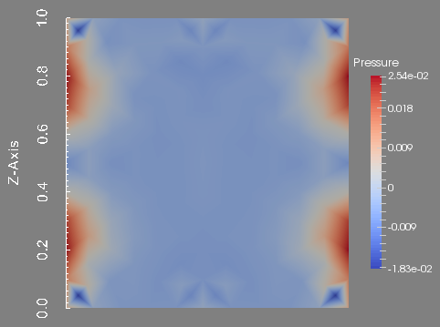
Pressure in the plane plane y=0.
|
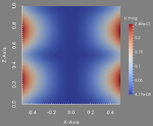
Velocity magnitude in the plane plane y=0.
|
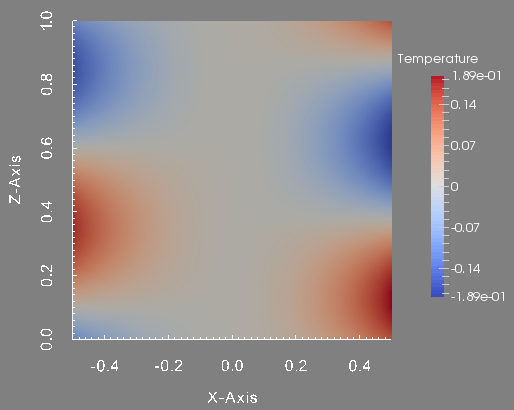
Temperature in the plane plane y=0.
|
 1.8.5
1.8.5 
