Introduction
In this example, we check the correctness of SFEMaNS for a magnetic problem involving a conducting domain. We consider Dirichlet and Neumann boundary conditions. We use P1 finite elements for the magnetic field.
We solve the Maxwell equations:
\begin{align} \begin{cases} \partial_t (\mu^c \mathbf{H}) + \nabla \times \left(\frac{1}{\Rm \sigma }\nabla \times \mathbf{H} \right) = \nabla\times (\bu^\text{given} \times \mu^c \mathbf{H}) + \nabla \times \left(\frac{1}{\Rm \sigma} \nabla\times \mathbf{j} \right) & \text{in } \Omega_1, \\ \text{div} (\mu^c \mathbf {H}) = 0 & \text{in } \Omega_1 ,\\ \bH \times \bn = \bH_{\text{bdy}} \times \bn & \text{on } \Gamma_1,\\ - \left( \frac{1}{\Rm \sigma} \left( \ROT (\mathbf{H}) - \mathbf{j} \right) - \bu^\text{given} \times \mu \mathbf{H} \right) = \textbf{a} \times \bn & \text{on } \Gamma_2,\\ \bH_{|t=0}= \bH_0, \end{cases} \end{align}
in the domain \(\Omega_1= \{ (r,\theta,z) \in {R}^3 : (r,\theta,z) \in [0,0.5] \times [0,2\pi) \times [0,1]\} \). We also set \(\Gamma_1= \partial \Omega_1\cap \{ z\in \{0,1\}\} \) and \(\Gamma_2= \partial \Omega_1 \cap \{ r=1\} \). The data are the source term \(\mathbf{j}\), the given velocity \(\bu^\text{given}\), the boundary datas \(\bH_{\text{bdy}}\) \(\textbf{a}\), the initial data \(\bH_0\). The parameter \(\Rm\) is the magnetic Reynolds number. The parameter \(\mu^c\) is the magnetic permeability of the conducting region \(\Omega_1\). The parameter \(\sigma\) is the conductivity in the conducting region \(\Omega_1\).
Manufactured solutions
We approximate the following analytical solutions:
\begin{align*} H_r(r,\theta,z,t) &= 0, \\ H_{\theta}(r,\theta,z,t) &= r - r^2 \sin(\theta), \\ H_z(r,\theta,z,t) &= r z \cos(\theta). \end{align*}
We also set the given velocity field as follows:
\begin{align*} u^\text{given}_r(r,\theta,z,t) &= 0, \\ u^\text{given}_{\theta}(r,\theta,z,t) &= 0, \\ u^\text{given}_z(r,\theta,z,t) &= 0. \end{align*}
The source term \( \mathbf{j} \) and the boundary datas \(\bH_{\text{bdy}}, \textbf{a}\) are computed accordingly.
Generation of the mesh
The finite element mesh used for this test is named Mesh_10_form.FEM and has a mesh size of \(0.1\) for the P1 approximation. You can generate this mesh with the files in the following directory: ($SFEMaNS_MESH_GEN_DIR)/EXAMPLES/EXAMPLES_MANUFACTURED_SOLUTIONS/Mesh_10_form. The following images show the mesh for P1 finite elements.
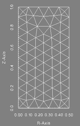
Finite element mesh (P1).
|
Information on the file condlim.f90
The initial conditions, boundary conditions and the forcing term \(\textbf{j}\) in the Maxwell equations are set in the file condlim_test_12.f90. Here is a description of the subroutines and functions of interest.
-
The subroutine
init_maxwell initializes the magnetic field and the scalar potential at the time \(-dt\) and \(0\) with \(dt\) being the time step. It is done by using the functions Hexact, Phiexact as follows: time = -dt
DO k=1,6
DO i=1, SIZE(list_mode)
Hn1(:,k,i) = Hexact(H_mesh,k, H_mesh%rr, list_mode(i), mu_H_field, time)
IF (inputs%nb_dom_phi>0) THEN
IF (k<3) THEN
phin1(:,k,i) = Phiexact(k, phi_mesh%rr, list_mode(i) , mu_phi, time)
ENDIF
END IF
ENDDO
ENDDO
time = time + dt
DO k=1,6
DO i=1, SIZE(list_mode)
Hn(:,k,i) = Hexact(H_mesh, k, H_mesh%rr, list_mode(i), mu_H_field, time)
IF (inputs%nb_dom_phi>0) THEN
IF (k<3) THEN
phin(:,k,i) = Phiexact(k, phi_mesh%rr, list_mode(i), mu_phi, time)
ENDIF
END IF
ENDDO
ENDDO
-
The function
Hexact contains the analytical magnetic field. It is used to initialize the magnetic field and to impose Dirichlet boundary conditions on \(\textbf{H}\times\textbf{n}\) with \(\textbf{n}\) the outter normal vector.
-
For the Fourier modes m∈{0,1}, we define the magnetic field depending of its TYPE (1 and 2 for the component radial cosine and sine, 3 and 4 for the component azimuthal cosine and sine, 5 and 6 for the component vertical cosine and sine) as follows:
IF (m==1) THEN
IF (TYPE==4) THEN
vv = -rr(1,:)**2
ELSE IF (TYPE==5) THEN
vv = rr(1,:)*rr(2,:)
ELSE
vv = 0.d0
END IF
ELSE IF (m==0) THEN
IF (TYPE==3) THEN
vv = rr(1,:)
ELSE IF (TYPE==5) THEN
vv = 0.d0
ELSE
vv = 0.d0
END IF
-
For the other Fourier modes, the magnetic field is set to zero.
ELSE
vv = 0.d0
END IF
RETURN
-
The function
Vexact is used to define the given velocity field \(\bu^\text{given}\). It is set to zero.
-
The function
Jexact_gauss is used to define the source term \(\textbf{j}\). Since \(\partial_t (\mu \textbf{H})=0\) and \( \bu^\text{given} \times \textbf{H}=0 \), we define this source term so it satisfies the relation \( \ROT\textbf{j}=\ROT(\ROT\textbf{H} )\). As this term only depends of the Fourier mode \(m=1\), we define it as follows: IF (m==1) THEN
IF (TYPE==2) THEN
vv = -rr(2)
ELSE IF (TYPE==3) THEN
vv = -rr(2)
ELSE IF (TYPE==6) THEN
vv = -3*rr(1)
ELSE
vv = 0.d0
END IF
ELSE
vv = 0.d0
END IF
RETURN
-
The function
Eexact_gauss is used to define the electric field \(\textbf{E}\). We remind that \( - \textbf{E}=\textbf{a} \times \textbf{n}\). In a conducting area, the electric field also satisfies the relation \(\textbf{E}= \frac{1}{\Rm \sigma} \left( \ROT (\mathbf{H}) - \mathbf{j} \right) - \bu^\text{given} \times (\mu \textbf{H}) \). It is defined as follows. IF (m/=0) THEN
vv = 0
ELSE
IF (TYPE==5) THEN
vv = 2.d0
ELSE
vv = 0.d0
END IF
END IF
RETURN
All the other subroutines present in the file condlim_test_12.f90 are not used in this test. We refer to the section Fortran file condlim.f90 for a description of all the subroutines of the condlim file.
Setting in the data file
We describe the data file of this test. It is called debug_data_test_12 and can be found in the following directory: ($SFEMaNS_DIR)/MHD_DATA_TEST_CONV_PETSC.
-
We use a formatted mesh by setting:
===Is mesh file formatted (true/false)?
.t.
-
The path and the name of the mesh are specified with the two following lines:
===Directory and name of mesh file
'.' 'Mesh_10_form.FEM'
-
We use two processors in the meridian section. It means the finite element mesh is subdivised in two.
===Number of processors in meridian section
2
-
We solve the problem for \(2\) Fourier modes.
===Number of Fourier modes
2
-
We use \(2\) processors in Fourier space.
===Number of processors in Fourier space
2
-
We select specific Fourier modes to solve.
===Select Fourier modes? (true/false)
-
We give the list of the Fourier modes to solve.
===List of Fourier modes (if select_mode=.TRUE.)
0 1
-
We approximate the Maxwell equations by setting:
===Problem type: (nst, mxw, mhd, fhd)
'mxw'
-
We do not restart the computations from previous results.
===Restart on velocity (true/false)
.f.
===Restart on magnetic field (true/false)
.f.
Vexact.
-
We use a time step of \(1\) and solve the problem over \(1\) time iterations.
===Time step and number of time iterations
1.d0, 1
-
We set the number of domains and their label, see the files associated to the generation of the mesh, where the code approximates the magnetic field.
===Number of subdomains in magnetic field (H) mesh
1
===List of subdomains for magnetic field (H) mesh
1
-
We set the number of interface in H_mesh.
===Number of interfaces in H mesh
0
-
We set the number of boundaries with Dirichlet conditions on the magnetic field and give their respective labels.
===Number of Dirichlet sides for Hxn
2
===List of Dirichlet sides for Hxn
2 4
-
We set the magnetic permeability in each domains where the magnetic field is approximated.
===Permeability in the conductive part (1:nb_dom_H)
1.d0
-
We set the conductivity in each domains where the magnetic field is approximated.
===Conductivity in the conductive part (1:nb_dom_H)
1.d0
-
We set the type of finite element used to approximate the magnetic field.
===Type of finite element for magnetic field
1
-
We set the magnetic Reynolds number \(\Rm\).
===Magnetic Reynolds number
1.d0
-
We set stabilization coefficient for the divergence of the magnetic field and the penalty of the Dirichlet and interface terms.
===Stabilization coefficient (divergence)
1.d0
===Stabilization coefficient for Dirichlet H and/or interface H/H
1.d0
-
We give information on how to solve the matrix associated to the time marching of the Maxwell equations.
-
===Maximum number of iterations for Maxwell solver
100
-
===Relative tolerance for Maxwell solver
1.d-6
===Absolute tolerance for Maxwell solver
1.d-10
-
===Solver type for Maxwell (FGMRES, CG, ...)
GMRES
===Preconditionner type for Maxwell solver (HYPRE, JACOBI, MUMPS...)
MUMPS
Outputs and value of reference
The outputs of this test are computed with the file post_processing_debug.f90 that can be found in the following: ($SFEMaNS_DIR)/MHD_DATA_TEST_CONV_PETSC.
To check the well behavior of the code, we compute three quantities:
-
The L2 norm of the error on the magnetic field \(\textbf{H}\).
-
The L2 norm of the error on the curl of the magnetic field \(\textbf{H}\).
-
The L2 norm of the divergence of the magnetic field \(\textbf{B}=\mu\bH\).
They are compared to reference values to attest of the correctness of the code. These values of reference are in the last lines of the file debug_data_test_12 in the directory ($SFEMaNS_DIR)/MHD_DATA_TEST_CONV_PETSC. They are equal to:
============================================
Mesh_10_form.FEM, P1
===Reference results
4.823924970280468E-003 L2 error on Hn
1.130509829567467E-002 L2 error on Curl(Hn)
4.821424313259546E-002 L2 norm of error on Div(mu Hn)
1. Dummy ref
To conclude this test, we show the profile of the approximated magnetic field \(\textbf{H}\) at the final time. This figure is done in the plane \(y=0\) which is the union of the half plane \(\theta=0\) and \(\theta=\pi\).
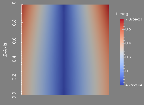
Magnetic field magnitude in the plane plane y=0.
|
 1.8.5
1.8.5 
