Introduction

In this example, we check the correctness of SFEMaNS for an eigenvalue problem of a magnetic set up. The set up involves a conducting domain only. We consider Dirichlet boundary conditions. We use P2 finite elements for the magnetic field.

We approximate the first five eigenvalues (with the largest real part) of the Maxwell equations:

\begin{align} \begin{cases} \partial_t (\mu^c \mathbf{H}) + \nabla \times \left(\frac{1}{\Rm \sigma}\nabla \times \mathbf{H} \right) = \nabla\times (\bu^\text{given} \times \mu^c \mathbf{H}) & \text{in } \Omega_1, \\ \text{div} (\mu^c \mathbf {H}) = 0 & \text{in } \Omega_1 ,\\ \bH \times \bn = \bH_{\text{bdy}} \times \bn & \text{on } \Gamma_1,\\ \bH_{|t=0}= \bH_0, \end{cases} \end{align}

in the conducting domain $\Omega_1= \{ (r,\theta,z) \in {R}^3 : (r,\theta,z) \in [0,1] \times [0,2\pi) \times [-1,1]\} $ with $\Gamma_1= \partial \Omega_1$. The data are the given velocity $\bu^\text{given}$, the boundary data $\bH_{\text{bdy}}$, the initial datas $\bH_0$. The parameter $\Rm$ is the magnetic Reynolds number. The parameter $\mu^c$ is the magnetic permeability of the conducting region $\Omega_1$. The parameter $\sigma$ is the conductivity in the conducting region $\Omega_1$.

Manufactured solutions

We consider the following solutions:

\begin{align*} H_r(r,\theta,z,t) &= A \frac{\sin(n_0z)}{r}(R_i-r)^2 (R_o-r)^2\cos(\theta), \\ H_{\theta}(r,\theta,z,t) &= -2 A \sin(n_0 z)(r-R_i)(r-R_o)(2r-R_o-R_i) \sin(\theta), \\ H_z(r,\theta,z,t) &= 0, \end{align*}

where $n_0=1$, $R_i=1$, $R_o=2$ and $A=10^{-3}$.

We also set the given velocity field as follows:

\begin{align*} u^\text{given}_r(r,\theta,z,t) &= - \text{amp}_{MND} \frac{\pi}{h} r (1-r^2)(1+2r) \cos(\frac{2\pi z}{h}), \\ u^\text{given}_{\theta}(r,\theta,z,t) &= \text{amp}_{MND}\frac{4\pi}{h} r (1-r) \sin^{-1}(z) , \\ u^\text{given}_z(r,\theta,z,t) &= \text{amp}_{MND} (1-r)(1+r+0.5 r^2)\sin(\frac{2\pi z}{h}), \end{align*}

where $\text{amp}_{MND}=1$ and $h=2$.

Generation of the mesh

The finite element mesh used for this test is named VKS_MND_form_10.FEM and has a mesh size of $0.1$ for the P1 approximation. You can generate this mesh with the files in the following directory: ($SFEMaNS_MESH_GEN_DIR)/EXAMPLES/EXAMPLES_MANUFACTURED_SOLUTIONS/VKS_MND_form_10. The following images show the mesh for P1 finite elements.

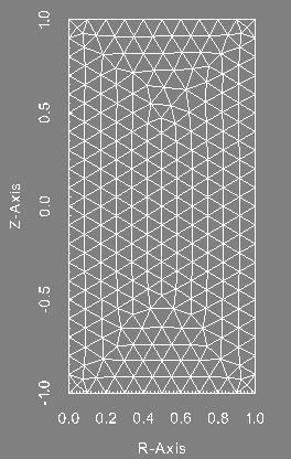
Finite element mesh (P1) of the conducting region.

Information on the file `condlim.f90`

The initial conditions, boundary conditions and the forcing term $\textbf{j}$ in the Maxwell equations are set in the file condlim_test_14.f90. Here is a description of the subroutines and functions of interest.

We define the real number $\pi$.
REAL(KIND=8) :: pi=ACOS(-1.d0)
The subroutine init_maxwell initializes the magnetic field at the time $-dt$ and $0$ with $dt$ being the time step. It is done as follows:
1. We set the magnetic fields to zero.
  time = 0.d0
  
  Hn = 0.d0
  
  Hn1 = 0.d0
  
  phin = 0.d0
  
  phin1 = 0.d0
  
  We note the scalar potential, not used in this test, is also initialized.
2. We define the parameters $n_0, R_i, R_0$ and $A$.
  n0 = 1
  
  Ri = 1.d0
  
  Ro = 2.d0
  
  A = 1d-3
3. For the Fourier mode $m=1$, we define the magnetic fields depending of their TYPE (1 and 2 for the component radial cosine and sine, 3 and 4 for the component azimuthal cosine and sine, 5 and 6 for the component vertical cosine and sine).
  IF (H_mesh%me /= 0) THEN
  
  DO i = 1, SIZE(list_mode)
  
  IF (list_mode(i) == 1) THEN
  
  Hn1(:,1,i) = A*(SIN(n0*H_mesh%rr(2,:))/H_mesh%rr(1,:))*(Ri-H_mesh%rr(1,:))**2 &
  
  * (Ro-H_mesh%rr(1,:))**2
  
  Hn(:,1,i) = A*(SIN(n0*H_mesh%rr(2,:))/H_mesh%rr(1,:))*(Ri-H_mesh%rr(1,:))**2 &
  
  * (Ro-H_mesh%rr(1,:))**2
  
  Hn1(:,4,i) = -2*A*SIN(n0*H_mesh%rr(2,:))*(H_mesh%rr(1,:)-Ri)&
  
  *(H_mesh%rr(1,:)-Ro)*(2.d0*H_mesh%rr(1,:)-Ro-Ri)
  
  Hn(:,4,i) = -2*A*SIN(n0*H_mesh%rr(2,:))*(H_mesh%rr(1,:)-Ri)&
  
  *(H_mesh%rr(1,:)-Ro)*(2.d0*H_mesh%rr(1,:)-Ro-Ri)
  
  END IF
  
  END DO
  
  END IF
  
  RETURN
  
  We note that Hn and Hn1 are equal (the problem is time independent).
The function Hexact is used to impose Dirichlet boundary conditions on $\textbf{H}\times\textbf{n}$ with $\textbf{n}$ the outter normal vector. It is set to zero as follows:
vv = 0.d0

RETURN
The function Vexact is used to define the given velocity field $\bu^\text{given}$.
1. We set the parameters $\epsilon, h, \zeta, \text{amp}_{MND}$ and $\text{amp}_{fl}$ used in the definition of the velocity field.
  REAL(KIND=8) :: eps=1.d-5, height=2.d0, zeta=30.d0, amp_MND=1.d0, amp_fl=0.d0
2. We set the velocity field to zero.
  vv = 0.d0
3. For the Fourier mode $m=0$, we define the velocity field depending of its TYPE (1 and 2 for the component radial cosine and sine, 3 and 4 for the component azimuthal cosine and sine, 5 and 6 for the component vertical cosine and sine).
  IF (m==0) THEN
  
  virgin = .TRUE.
  
  DO mjl = 1, H_mesh%me
  
  !IF (H_mesh%i_d(mjl)/= 4) CYCLE
  
  !We are in the sodium
  
  DO njl = 1, H_mesh%gauss%n_w
  
  i = H_mesh%jj(njl,mjl)
  
  IF (.NOT.virgin(i)) CYCLE
  
  virgin(i) = .FALSE.
  
  rr = H_mesh%rr(1,i)
  
  zz = H_mesh%rr(2,i)
  
  vv(i,1) = amp_MND*(-(PI/height)*rr*(1.d0-rr)**2*(1.d0+2.d0*rr)*COS(2.d0*PI*zz/height))
  
  vv(i,3) = amp_MND*(4.d0*height/PI)*rr*(1.d0-rr)*ASIN(zz)
  
  IF (zz .LE. (-eps)) THEN ! On est en bas
  
  vv(i,3) = vv(i,3)+ amp_fl*rr*SIN(PI*rr)*(1.-2.*zeta*(zz+1.)**2)*EXP(-zeta*(zz+1.)**2)
  
  ELSE IF (zz .GE. eps) THEN ! On est en haut
  
  vv(i,3) = vv(i,3)+ amp_fl*rr*SIN(PI*rr)*(1.-2.*zeta*(zz-1.)**2)*EXP(-zeta*(zz-1.)**2)
  
  ENDIF
  
  vv(i,5) = amp_MND*(1.-rr)*(1.+rr-5.*rr**2)*SIN(2.*PI*zz/height)
  
  !!$ vel_loc(i) = sqrt(vv(i,1)**2 + vv(i,3)**2 + vv(i,5)**2)
  
  END DO !njl
  
  END DO
  
  END IF
  
  We note that the part multiphy by amp_fl is equal to zero. As a result, the parameters $\epsilon$, $\zeta$ and $\text{amp}_{nl}$ could be removed from this function.
The function Jexact_gauss is used to define the source term $\textbf{j}$ that is not used in this test. It is set to zero.
vv = 0.d0

RETURN

All the other subroutines present in the file condlim_test_14.f90 are not used in this test. We refer to the section Fortran file condlim.f90 for a description of all the subroutines of the condlim file.

Setting in the data file

We describe the data file of this test. It is called debug_data_test_14 and can be found in the following directory: ($SFEMaNS_DIR)/MHD_DATA_TEST_CONV_PETSC.

We use a formatted mesh by setting:
===Is mesh file formatted (true/false)?

.t.
The path and the name of the mesh are specified with the two following lines:
===Directory and name of mesh file

'.' 'VKS_MND_form_10.FEM'

where '.' refers to the directory where the data file is, meaning ($SFEMaNS_DIR)/MHD_DATA_TEST_CONV_PETSC.
We use one processor in the meridian section. It means the finite element mesh is not subdivised.
===Number of processors in meridian section

1
We solve the problem for $2$ Fourier modes.
===Number of Fourier modes

2
We use $2$ processors in Fourier space.
===Number of processors in Fourier space

2

It means that each processors is solving the problem for $2/2=1$ Fourier modes.
We do not select specific Fourier modes to solve.
===Select Fourier modes? (true/false)

.f.
We give the list of the Fourier modes to solve.
===Problem type: (nst, mxw, mhd, fhd)

'mxw'

===Restart on velocity (true/false)

.f.
We do not restart the computations from previous results.
===Restart on velocity (true/false)

.f.

===Restart on magnetic field (true/false)

.f.

It means the computation starts from the time $t=0$. We note that we need to say if we use a restart for the velocity. If yes, the $\bu^\text{given}$ comes from a suite file and not the function Vexact.
We use a time step of $0.01$ and solve the problem over one time iteration.
===Time step and number of time iterations

1.d-2, 1
To solve an eigenvalue problem with arpack we need to set the following parameters.
1. We use arpack.
  ===Do we use Arpack?
  
  .t.
2. We set the number of eigenvalues to compute.
  ===Number of eigenvalues to compute
  
  5
3. We set the maximum number of iterations Arpack can do.
  ===Maximum number of Arpack iterations
  
  3000
4. We set the tolerance.
  ===Tolerance for Arpack
  
  1.d-3
5. We give information on which eigenvalues we are looking for.
  ===Which eigenvalues ('LM', 'SM', 'SR', 'LR' 'LI', 'SI')
  
  'LR'
  
  We note that "LM", "SM", "SR", "LR", "LI" and "SI" respectively means largest magnitude, smallest magnitude, smallest real part, largest real part, largest imaginary part and smallest imaginary part.
6. We generate vtu files with the following option.
  ===Create 2D vtu files for Arpack? (true/false)
  
  .t.
We set the number of domains and their label, see the files associated to the generation of the mesh, where the code approximates the magnetic field.
===Number of subdomains in magnetic field (H) mesh

1

===List of subdomains for magnetic field (H) mesh

1
We set the number of interface in H_mesh.
===Number of interfaces in H mesh

0

Such interfaces represent interfaces with discontinuities in magnetic permeability or interfaces between the magnetic field mesh and the temperature or the velocity field meshes.
We set the number of boundaries with Dirichlet conditions on the magnetic field and give their respective labels.
===Number of Dirichlet sides for Hxn

3

===List of Dirichlet sides for Hxn

2 4 3
We set the magnetic permeability in each domains where the magnetic field is approximated.
===Permeability in the conductive part (1:nb_dom_H)

1.d0
We set the conductivity in each domains where the magnetic field is approximated.
===Conductivity in the conductive part (1:nb_dom_H)

1.d0
We set the type of finite element used to approximate the magnetic field.
===Type of finite element for magnetic field

2
We set the magnetic Reynolds number $\Rm$.
===Magnetic Reynolds number

80.d0
We set stabilization coefficient for the divergence of the magnetic field and the penalty of the Dirichlet and interface terms.
===Stabilization coefficient (divergence)

1.d0

===Stabilization coefficient for Dirichlet H and/or interface H/H

1.d0

We note these coefficients are usually set to $1$.
We give information on how to solve the matrix associated to the time marching of the Maxwell equations.
1. ===Maximum number of iterations for Maxwell solver
  
  100
2. ===Relative tolerance for Maxwell solver
  
  1.d-6
  
  ===Absolute tolerance for Maxwell solver
  
  1.d-10
3. ===Solver type for Maxwell (FGMRES, CG, ...)
  
  GMRES
  
  ===Preconditionner type for Maxwell solver (HYPRE, JACOBI, MUMPS...)
  
  MUMPS
To get the total elapse time and the average time in loop minus initialization, we write:
===Verbose timing? (true/false)

.t.

These informations are written in the file lis when you run the shell debug_SFEMaNS_template.

Outputs and value of reference

The outputs of this test are computed with the file post_processing_debug.f90 that can be found in the following directory: ($SFEMaNS_DIR)/MHD_DATA_TEST_CONV_PETSC.

To check the well behavior of the code, we compute four quantities:

The real part of the first eigenvalue of the mode 0.
The relative divergence of the first eigenvalue of the mode 0.
The real part of the first eigenvalue of the mode 1.
The relative divergence of the first eigenvalue of the mode 1.

They are compared to reference values to attest of the correctness of the code. These values of reference are in the last lines of the file debug_data_test_14 in the directory ($SFEMaNS_DIR)/MHD_DATA_TEST_CONV_PETSC. They are equal to: