Introduction
In this example, we check the correctness of SFEMaNS for a hydrodynamic problem of a precession set up involving Neumann boundary conditions. The main rotation axis is the vertical axis while the precession axis is along the unit normal vector \(\textbf{e}_x\) associated to the x cartesian coordinate. The computation is done in the precession frame, meaning the walls only see the main rotation along the vertical axis. We note this test does not involve manufactured solution and consist to check four quantities, like the total kinetic energy, are the same than the values of reference.
We solve the Navier-Stokes equations:
\begin{align*} \partial_t\bu+\left(\ROT\bu + 2 \epsilon \textbf{e}_x \right)\CROSS\bu - \frac{1}{\Re}\LAP \bu +\GRAD p &=0, \\ \DIV \bu &= 0, \\ \bu \cdot \textbf{n}_{|\Gamma} &= 0, \\ \bu_{|t=0} &= \bu_0, \\ p_{|t=0} &= p_0, \end{align*}
in the domain \(\Omega= \{ (r,\theta,z) \in {R}^3 : (r,\theta,z) \in [0,1] \times [0,2\pi) \times [0,.8]\; | \; r^2 + \frac{z^2}{0.8^2} =1\} \) with \(\Gamma= \partial \Omega \). The data are the initial datas \(\bu_0\) and \(p_0\). The parameter \(\Re\) is the kinetic Reynolds number, \(\epsilon\) is the precession rate and \(\alpha\) is the precession angle.
Manufactured solutions
As mentionned earlier this test does not involve manufactured solutions. As consequence we do not consider specific source term and only initialize the variables to approximate.
\begin{align*} u_r(r,\theta,z,t=0) &= 0, \\ u_{\theta}(r,\theta,z,t=0) &= 0.1r, \\ u_z(r,\theta,z,t=0) &=0, \\ p(r,\theta,z,t=0) &= \frac{(0.1 r)^2}{2} . \end{align*}
Generation of the mesh
The finite element mesh used for this test is named ELL_b0p8_10_form.FEM. The mesh size for the P1 approximation \(0.1\) on the boundary of the domain and \(0.033\) at \((r,z)=(0,0)\). You can generate this mesh with the files in the following directory: ($SFEMaNS_MESH_GEN_DIR)/EXAMPLES/EXAMPLES_MANUFACTURED_SOLUTIONS/ELL_b0p8_10_form. The following image shows the mesh for P1 finite elements.
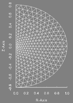
Finite element mesh (P1).
|
Information on the file condlim.f90
The initial conditions, boundary conditions and the forcing term \(\textbf{f}\) in the Navier-Stokes equations are set in the file condlim_test_16.f90. Here is a description of the subroutines and functions of interest.
-
The subroutine
init_velocity_pressure initializes the velocity field and the pressure at the time \(-dt\) and \(0\) with \(dt\) being the time step. It is done by using the functions vv_exact and pp_exact as follows: time = 0.d0
DO i= 1, SIZE(list_mode)
mode = list_mode(i)
DO j = 1, 6
!===velocity
un_m1(:,j,i) = vv_exact(j,mesh_f%rr,mode,time-dt)
un (:,j,i) = vv_exact(j,mesh_f%rr,mode,time)
END DO
DO j = 1, 2
!===pressure
pn_m2(:) = pp_exact(j,mesh_c%rr,mode,time-2*dt)
pn_m1 (:,j,i) = pp_exact(j,mesh_c%rr,mode,time-dt)
pn (:,j,i) = pp_exact(j,mesh_c%rr,mode,time)
phin_m1(:,j,i) = pn_m1(:,j,i) - pn_m2(:)
phin (:,j,i) = Pn (:,j,i) - pn_m1(:,j,i)
ENDDO
ENDDO
-
The function
vv_exact contains the analytical velocity field. It is used to initialize the velocity field.
-
First we define the radial and vertical coordinates r, z.
-
For a time strictly larger than 0, we set the valocity field to zero. We note that the above line are not required since this test does not involved Dirichlet boundary conditions. As a consequence this function is only used to initialize the velocity field.
-
If the Fourier mode m is not equal to 0, the velocity field is set to zero.
ELSE
IF (m/=0) THEN
vv = 0.d0
-
For the Fourier mode \(m=0\), we define the velocity field depending of its TYPE (1 and 2 for the component radial cosine and sine, 3 and 4 for the component azimuthal cosine and sine, 5 and 6 for the component vertical cosine and sine) as follows:
ELSE
IF (TYPE==3) THEN
vv = 0.1d0*r
ELSE
vv = 0.d0
END IF
END IF
END IF
RETURN
-
The function
pp_exact contains the analytical pressure. It is used to initialize the pressure.
-
First we define the radial and vertical coordinates r, z.
-
For a time strictly larger than 0, we set the pressure to zero. We note that the above line are not required since this function is only used to initialize the pressure.
-
If the Fourier mode m is not equal to 0, the pressure is set to zero.
-
For the Fourier mode \(m=0\), we define the pressure depending of its TYPE (1 for cosine and 2 for sine) as follows:
ELSE
IF (TYPE==1) THEN
vv = (0.1d0*r)**2/2.d0
ELSE
vv = 0.d0
END IF
END IF
END IF
RETURN
-
The function
source_in_NS_momentumis used to define the source term \(\bef\) of the Navier-Stokes equations. As this term is not used for this test, it is set to zero.
All the other subroutines present in the file condlim_test_16.f90 are not used in this test. We refer to the section Fortran file condlim.f90 for a description of all the subroutines of the condlim file.
Setting in the data file
We describe the data file of this test. It is called debug_data_test_16 and can be found in the following directory: ($SFEMaNS_DIR)/MHD_DATA_TEST_CONV_PETSC.
-
We use a formatted mesh by setting:
===Is mesh file formatted (true/false)?
.t.
-
The path and the name of the mesh are specified with the two following lines:
===Directory and name of mesh file
'.' 'ELL_b0p8_10_form.FEM'
-
We use two processors in the meridian section. It means the finite element mesh is subdivised in two. To do so, we write:
===Number of processors in meridian section
2
-
We solve the problem for \(8\) Fourier modes.
===Number of Fourier modes
8
-
We use \(4\) processors in Fourier.
===Number of processors in Fourier space
4
-
We do not select specific Fourier modes to solve.
===Select Fourier modes? (true/false)
-
We approximate the Navier-Stokes equations by setting:
===Problem type: (nst, mxw, mhd, fhd)
'nst'
-
We do not restart the computations from previous results.
===Restart on velocity (true/false)
.f.
-
We use a time step of \(0.1\) and solve the problem over \(20\) time iterations.
===Time step and number of time iterations
1d-1, 20
-
We set the number of domains and their label, see the files associated to the generation of the mesh, where the code approximates the Navier-Stokes equations,
===Number of subdomains in Navier-Stokes mesh
1
===List of subdomains for Navier-Stokes mesh
1
-
We set the number of boundaries with Dirichlet conditions on the velocity field.
===How many
boundary pieces
for full Dirichlet BCs on velocity?
0
-
We set the number of boundaries with homogeneous Neumann conditions on the velocity field and give their respective labels.
===How many
boundary pieces
for homogeneous normal velocity?
1
===List of
boundary pieces
for homogeneous normal velocity
2
-
We set the kinetic Reynolds number \(\Re\).
-
We want to add the term \( 2\epsilon \textbf{e}_x \times \bu \) in the left hand side of the Navier-Stokes equations. Such features is already programmed in SFEMaNS via the following lines in your data file.
-
We set the option precession to true.
===Is there a precession term (true/false)?
.t.
-
We set the precession rate \(\epsilon\) and the precesion angle \(\alpha\).
===Precession rate
0.25d0
===Precession angle over pi
0.5d0
-
We give information on how to solve the matrix associated to the time marching of the velocity.
-
===Maximum number of iterations for velocity solver
100
-
===Relative tolerance for velocity solver
1.d-6
===Absolute tolerance for velocity solver
1.d-10
-
===Solver type for velocity (FGMRES, CG, ...)
GMRES
===Preconditionner type for velocity solver (HYPRE, JACOBI, MUMPS...)
MUMPS
-
We give information on how to solve the matrix associated to the time marching of the pressure.
-
===Maximum number of iterations for pressure solver
100
-
===Relative tolerance for pressure solver
1.d-6
===Absolute tolerance for pressure solver
1.d-10
-
===Solver type for pressure (FGMRES, CG, ...)
GMRES
===Preconditionner type for pressure solver (HYPRE, JACOBI, MUMPS...)
MUMPS
-
We give information on how to solve the mass matrix.
-
===Maximum number of iterations for mass matrix solver
100
-
===Relative tolerance for mass matrix solver
1.d-6
===Absolute tolerance for mass matrix solver
1.d-10
-
===Solver type for mass matrix (FGMRES, CG, ...)
CG
===Preconditionner type for mass matrix solver (HYPRE, JACOBI, MUMPS...)
MUMPS
-
To get the total elapse time and the average time in loop minus initialization, we write:
===Verbose timing? (true/false)
lis when you run the shell debug_SFEMaNS_template.
Outputs and value of reference
The outputs of this test are computed with the file post_processing_debug.f90 that can be found in the following directory: ($SFEMaNS_DIR)/MHD_DATA_TEST_CONV_PETSC.
To check the well behavior of the code, we compute four quantities:
-
The total kinetic energy \( \displaystyle 0.5 {\Vert \bu \Vert}_{\bL^2(\Omega)}^2\).
-
The quantity \(M_x= \displaystyle \int_\Omega \left(-z(\sin(\theta)u_r + \cos(\theta) u_\theta) +r \sin(\theta)u_z \right) r dr d\theta dz\).
-
The quantity \(M_y= \displaystyle \int_\Omega \left(z(\cos(\theta)u_r - \sin(\theta) u_\theta ) -r \cos(\theta)u_z \right) r dr d\theta dz\).
-
The quantity \(M_z= \displaystyle \int_\Omega u_\theta r^2 dr d\theta dz \).
These quantities are computed at the final time \(t=2\). We note the last three quantities are computed via the subroutine angular_momentum of the file tn_axi.f90. They are compared to reference values to attest of the correctness of the code. These values of reference are in the last lines of the file debug_data_test_16 in the directory ($SFEMaNS_DIR)/MHD_DATA_TEST_CONV_PETSC. They are equal to:
============================================
ELL_b0p8_10_form.FEM, dt=1d-1, it_max=20
===Reference results
6.67555315567430665E-003 !Total kinetic energy at
t=2
9.61565539080621234E-004 !Mx
4.87365427729861689E-002 !My
0.12184513917556984 !Mz
To conclude this test, we show the profile of the approximated pressure and velocity magnitude at the final time. These figures are done in the plane \(y=0\) which is the union of the half plane \(\theta=0\) and \(\theta=\pi\).
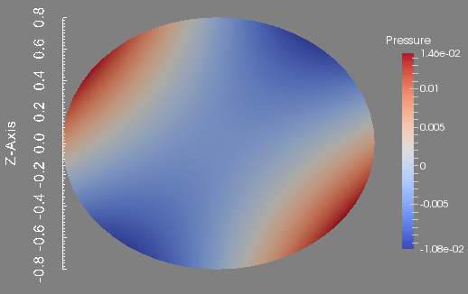
Pressure in the plane plane y=0.
|
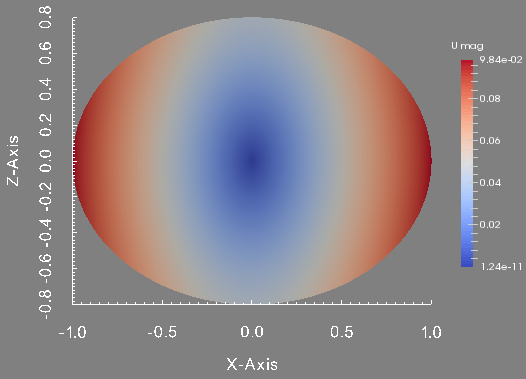
Velocity magnitude in the plane plane y=0.
|
 1.8.5
1.8.5 
