Introduction
In this example, we check the correctness of SFEMaNS for stationary magnetic problem involving a conducting. The magnetic permeability is variable in \((r,,\theta,z)\) and presents a jump in \(r=1\). The magnetic permeability is given. We consider Dirichlet boundary conditions. We use P2 finite elements. This set up is approximated over one time iterations with a large time step.
We solve the Maxwell equations with the magnetic field \(\bB=\mu \bH\) as dependent variable:
\begin{align} \begin{cases} \partial_t (\mathbf{B}) + \nabla \times \left(\frac{1}{\Rm \sigma}\nabla \times( \frac{1}{\mu^c}\mathbf{B} ) \right) = \nabla\times (\bu^\text{given} \times \mathbf{B}) + \nabla \times \left(\frac{1}{\Rm \sigma} \nabla\times \mathbf{j} \right) & \text{in } \Omega, \\ \text{div} (\mathbf{B}) = 0 & \text{in } \Omega ,\\ \bH_1 \times \bn_1 + \bH_2 \times \bn_2 = 0 & \text{on } \Sigma_\mu,\\ \mu^c_1\bH _1 \cdot \bn_1 + \mu^c_2 \bH _2 \cdot \bn_2 = 0 & \text{on } \Sigma_\mu,\\ {\bH \times \bn}_{|\Gamma} = {\bH_{\text{bdy}} \times \bn}_{|\Gamma}, &\\ \bH_{|t=0}= \bH_0, \\ \end{cases} \end{align}
in the domain \(\Omega= \{ (r,\theta,z) \in {R}^3 : (r,\theta,z) \in [0,2] \times [0,2\pi) \times [0.25,1]\} \). This domain is the union of two conduction domain \(\Omega_1=\{ (r,\theta,z) \in {R}^3 : (r,\theta,z) \in [0,1] \times [0,2\pi) \times [0.25,1]\}\) and \( \Omega_2= \{ (r,\theta,z) \in {R}^3 : (r,\theta,z) \in [1,2] \times [0,2\pi) \times [0.25,1]\}\). We denote by \(\Sigma_\mu\) the interface of \(\Omega_1\) and \(\Omega_2\). We also set \(\Gamma= \partial \Omega\). We define outward normals \(\bn_1, \bn_2\) to the surface \(\Sigma_\mu\) and the outward normals \(\bn\) to the surface \(\Gamma\). The data are the source term \(\mathbf{j}\), the given velocity \(\bu^\text{given}\), the boundary data \(\bH_{\text{bdy}}\) and the initial data \(\bH_0\). The parameter \(\Rm\) is the magnetic Reynolds number. The parameter \(\mu^c\) is the magnetic permeability of the conducting region \(\Omega\). The parameter \(\sigma\) is the conductivity in the conducting region \(\Omega\).
Manufactured solutions
We define the magnetic permeability in the conducting region as follows:
\begin{align*} \mu^c(r,z)= \begin{cases} \frac{1}{ 1 + f_{23}(r,z) \cos(m_{23}\theta) } & \text{ in } \Omega_1, \\ \frac{1+\lambda_\mu/z}{ 1 + f_{23}(r,z) \cos(m_{23}\theta)} &\text{ in } \Omega_2, \end{cases} \end{align*}
with \(lambda_\mu= 1\), \(m_{23}=3\) and \(f_{23}\) defined as follows:
\begin{align*} f_{23}(r,z)=\frac{1}{0.00016}\frac{\text{ratio}_\mu-1}{\text{ratio}_\mu+1} \left(r(1-r)(r-2)(z-0.25)(z-1)\right)^3, \end{align*}
where \(\text{ratio}_\mu=50\) represents the fraction of the minimum over the maximum of the magnetic permeability in the conducting region.
We approximate the following analytical solutions:
\begin{align*} H_r(r,\theta,z,t) &= \begin{cases} r ( 1 + f_{23}(r,z) \cos(m_{23}\theta)) & \text{ in } \Omega_1, \\ \frac{r}{1+\lambda_\mu/z} ( 1 + f_{23}(r,z) \cos(m_{23}\theta)) &\text{ in } \Omega_2, \end{cases} \\ H_{\theta}(r,\theta,z,t) &=0, \\ H_z(r,\theta,z,t) &= \begin{cases} -2 z ( 1 + f_{23}(r,z) \cos(m_{23}\theta)) & \text{ in } \Omega_1, \\ 0 &\text{ in } \Omega_2. \end{cases} \end{align*}
and remind that \(\bB=\mu\bH\).
We also set the given velocity field to zero.
\begin{align*} u^\text{given}_r(r,\theta,z,t) &= 0, \\ u^\text{given}_{\theta}(r,\theta,z,t) &= 0, \\ u^\text{given}_z(r,\theta,z,t) &= 0. \end{align*}
The source term \( \mathbf{j}\) and the boundary data \(\bH_{\text{bdy}}\) are computed accordingly.
Generation of the mesh
The finite element mesh used for this test is named mesh_18_0.025.FEM. The mesh size for the P1 approximation is \(0.025\) in \(\Omega\). You can generate this mesh with the files in the following directory: ($SFEMaNS_MESH_GEN_DIR)/EXAMPLES/EXAMPLES_MANUFACTURED_SOLUTIONS/mesh_18_0.05.FEM (after editing the topology files). The following images show the mesh for P1 finite elements for the conducting and vacuum regions.
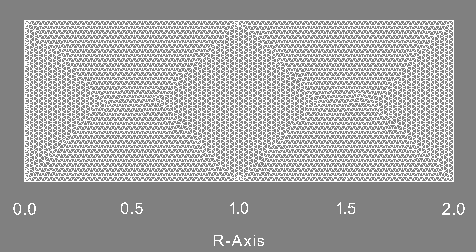
Finite element mesh (P1) of the conducting region.
|
Information on the file condlim.f90
The initial conditions, boundary conditions and the forcing term \(\textbf{j}\) in the Maxwell equations are set in the file condlim_test_23.f90. This condlim also uses functions of the file test_23.f90 to define the magnetic permeability and its gradient. Here is a description of the subroutines and functions of interest of the file condlim_test_23.f90.
-
The subroutine
init_maxwell initializes the magnetic field at the time \(-dt\) and \(0\) with \(dt\) being the time step. It is set to zero as follows: Hn1 = 0.d0
Hn = 0.d0
phin1 = 0.d0
phin = 0.d0
time=0.d0
RETURN
-
The function
Hexact contains the analytical magnetic field. It is used to impose Dirichlet boundary conditions on \(\textbf{H}\times\textbf{n}\) with \(\textbf{n}\) the outter normal vector.
-
We define a tabular id so that each nodes n, id(n) is equal to 1 or 2 depending if the node is in \(\Omega_1\) or \(\Omega_2\).
-
If rr contains the radial and vertical coordinates of each np nodes, we define id as follows.
IF (SIZE(rr,2)== H_mesh%np) THEN
DO mm = 1, H_mesh%me !id is used to determine on which side of the interface we are
END DO
-
If rr does not contain the information on np nodes, it means Hexact is called to set boundary conditions. In that case, Hexact is called one time per nodes. So we define id, a tabular of dimension 1, as follows:
ELSE
IF (rr(1,1)<1) THEN !used for
boundary condition
id = 1
ELSE
id = 2
END IF
END IF
-
For the Fourier mode \(m=0\) and \(m=m_{23}\), we define the magnetic field depending of its TYPE (1 and 2 for the component radial cosine and sine, 3 and 4 for the component azimuthal cosine and sine, 5 and 6 for the component vertical cosine and sine) and the subdomain considered follows:
DO n = 1, SIZE(rr,2)
IF (m == 0) THEN
IF (TYPE==1) THEN
IF(id(n)==1) THEN
vv(n) = rr(1,n)
ELSE
vv(n) = rr(1,n)/(1.d0 + lambda_mu_T23/rr(2,n) )
END IF
ELSE IF (TYPE==5) THEN
vv(n) = -2.d0*rr(2,n)
ELSE
vv(n) = 0.d0
END IF
ELSE IF (m == mode_mu_T23) THEN
IF (TYPE==1) THEN
IF(id(n)==1) THEN
vv(n) = rr(1,n)*s_test_T23(rr(1,n),rr(2,n))
ELSE
vv(n) = rr(1,n)*s_test_T23(rr(1,n),rr(2,n))/(1.d0 + lambda_mu_T23/rr(2,n))
END IF
ELSE IF (TYPE==5) THEN
vv(n) = -2.d0*rr(2,n)*s_test_T23(rr(1,n),rr(2,n))
ELSE
vv(n) = 0.d0
END IF
ELSE
vv = 0.d0
END IF
END DO
RETURN
test_23.f90.
-
The function
Vexact is used to define the given velocity field \(\bu^\text{given}\). It is set to zero.
-
The function
Jexact_gauss is used to define the source term \(\textbf{j}\). We remind that \( \bu^\text{given}=0 \) and \(\partial_t \textbf{H}=0\) so it is defined such that \(\textbf{j}=\ROT \bH\).
-
First we define the cylindrical coordinates (r,z) of the node considered.
-
For the Fourier mode \(m=0\), the azimuthal component of \(\textbf{j}\) in the domain \(\Omega_2\) is defined as follows:
!DCQ: mesh_id gives us now info about what side (domain) we are.
IF ((m==0) .AND. (mesh_id==2) .AND. (TYPE==3)) THEN
!J_theta
beta=lambda_mu_T23/((1.d0 + lambda_mu_T23/
z)**2 *
z**2)
vv=r*beta
-
For the Fourier mode \(m=m_{23}\), the source term is defined of its TYPE (1 and 2 for the component radial cosine and sine, 3 and 4 for the component azimuthal cosine and sine, 5 and 6 for the component vertical cosine and sine) and the subdomain considered (mesh_id=1 in \(\Omega_1\) and 2 in \(\Omega_2\)).
ELSE IF (m==mode_mu_T23) THEN
!J_r
IF (TYPE==2) THEN
vv = 2.d0*m*
z*b_factor_T23*r**2*( (r-1.d0)*(r-2.d0)*(
z-0.25)*(
z-1.d0) )**3
!J_theta
ELSE IF (TYPE==3) THEN
alpha =6*b_factor_T23*
z*( (
z-0.25)*(
z-1) )**3*( r* (r-1.d0)*(r-2.d0) )**2 &
*( r*(r-1)+r*(r-2)+(r-1)*(r-2))
IF (mesh_id==1) THEN
vv= 3*b_factor_T23*r**4*( (r-1)*(r-2) )**3 *( (
z-0.25)*(
z-1) )**2&
*( 2*
z -1 - 0.25) + alpha
ELSE
beta =lambda_mu_T23/((1.d0 + lambda_mu_T23/
z)**2 *
z**2)
vv= b_factor_T23*r**4*( (r-1.d0)*(r-2.d0) )**3 *( (
z-0.25)*(
z-1) )**2 &
*( 3*(2*
z- 1 - 0.25 )/(1.d0+lambda_mu_T23/
z) + beta*(
z-1)*(
z-0.25) ) &
+ alpha
END IF
!J_z
ELSE IF (TYPE==6) THEN
IF (mesh_id==1) THEN
ELSE
vv = m*s_test_T23(r,
z)/(1.d0+lambda_mu_T23/
z)
ENDIF
ELSE
vv = 0.d0
END IF
ELSE
vv = 0.d0
END IF
RETURN
-
The function
mu_bar_in_fourier_space defines a stabilization term, denoted mu_bar, on the nodes or gauss points of the finite element mesh. It needs to be smaller than mu everywhere in the domain. It is done by using the function mu_bar_in_fourier_space_anal_T23 of the file test_23.f90. IF( PRESENT(pts) .AND. PRESENT(pts_ids) ) THEN
vv=mu_bar_in_fourier_space_anal_T23(H_mesh,nb,ne,pts,pts_ids)
ELSE
vv=mu_bar_in_fourier_space_anal_T23(H_mesh,nb,ne)
END IF
RETURN
-
The function
grad_mu_bar_in_fourier_space defines the gradient of mu_bar. It is done by using the function grad_mu_bar_in_fourier_space_anal_T2 of the file test_22.f90. vv=grad_mu_bar_in_fourier_space_anal_T23(pt,pt_id)
RETURN
-
The function
mu_in_real_space defines the magnetic permeability. It is done by using the function mu_in_real_space_anal_T23 of the file test_23.f90. vv = mu_in_real_space_anal_T23(H_mesh,angles,nb_angles,nb,ne)
RETURN
All the other subroutines present in the file condlim_test_23.f90 are not used in this test. We refer to the section Fortran file condlim.f90 for a description of all the subroutines of the condlim file. The following describes the functions of interest of the file test_23.f90.
-
First we define the real numbers \(ratio_\mu\), \(b\), \(\lambda_\mu\) and the interger \(m_{23}\).
REAL (kind=8),PARAMETER, PUBLIC :: ratio_mu_T23 = 50.0d0 ! the variation of mu1
REAL (kind=8), PUBLIC :: b_factor_T23 = (1.d0/0.00016) * (ratio_mu_T23 - 1.d0)/(ratio_mu_T23 +1.d0)
REAL (kind=8), PUBLIC :: lambda_mu_T23 = 1.d0
INTEGER, PUBLIC :: mode_mu_T23 = 3
-
The function
s_test_T23 defines the function \(f_{23}\). vv = b_factor_T23*( r*(r-1.d0)*(r-2.d0)*(
z-0.25)*(
z-1.d0) )**3
RETURN
-
The function
Ds_test_T23 defines the gradient of the function \(f_{23}\).
-
We compute the r-derivative as follows:
vv(1) = b_factor_T23*((
z-0.25)*(
z-1.d0))**3 * &
( 3*( r*(r-1.d0)*(r-2.d0) )**2*( r*( (r-1)+(r-2) ) + (r-1)*(r-2) ) )
-
We compute the z-derivative as follows:
vv (2) = b_factor_T23*( r*(r-1.d0)*(r-2.d0))**3 * &
( 3* (
z-0.25)*(
z-1.d0) )**2 *( (
z-1.d0) + (
z-0.25) )
RETURN
-
The function
mu_bar_in_fourier_space_anal_T23 defines stabilization term mu_bar such that it is smaller than mu everywhere in the domain.
-
First we define the radial and vertical cylindrical coordinates of each nodes. We also define a tabular local_ids that is equal to 1 if the node is in \(\Omega_1\) and 2 if it's in \(\Omega_2\).
IF( PRESENT(pts) .AND. PRESENT(pts_ids) ) THEN !Computing mu at pts
r=pts(1,nb:ne)
local_ids=pts_ids
ELSE
r=H_mesh%rr(1,nb:ne) !Computing mu at nodes
DO m = 1, H_mesh%me
global_ids(H_mesh%jj(:,m)) = H_mesh%i_d(m)
END DO
local_ids=global_ids(nb:ne)
END IF
-
We define the stabilization term mu_bar.
DO n = 1, ne - nb + 1
s = s_test_T23(r(n),
z(n))
IF(local_ids(n)==1) THEN
vv(n) = 1.d0/(1.d0 + ABS(s)) !mu1_bar, DCQ: If you change mu1_bar, you have to change
!Jexact_gauss() as well
ELSE
vv(n) = 1.d0/( (1.d0 + ABS(s)))*(1.d0 + lambda_mu_T23/
z(n)) !mu2_bar
END IF
END DO
RETURN
-
The function
grad_mu_bar_in_fourier_space_anal_T23 defines the gradient of mu_bar on gauss points.
-
We define the radial and vertical cylindrical coordinates (r,z).
-
We compute \(f_{23}(r,z)\) and define a function sign depending of its value.
IF (s .GE. 0.d0 ) THEN
sign =1.0
ELSE
sign =-1.0
END IF
-
We compute the gradient of \(f_{23}\) in (r,z).
tmp=Ds_test_T23(r,
z)!derivative
-
We define the gradient of mu_bar.
IF(pt_id(1)==1) THEN !grad_mu_1
vv(1)= 1.d0
vv(2)= 0.d0
ELSE !grad_mu_2
vv(1)=1.d0 + ( (3*r+2)*(2*lambda_mu_T23) - ( (2*lambda_mu_T23*(1+r)))*(3) ) /(
z*(3*r+2) )**2
vv(2)= (2*lambda_mu_T23*(1+r))/(3*r+2)*(-2/
z**3)
END IF
RETURN
-
The function
mu_in_real_space_anal_T23 defines the magnetic permeability (depending of the node in the meridian plan and its angle).
-
We define a tabular id that is equal to 1 if the node is in \(\Omega_1\) and 2 if it's in \(\Omega_2\).
DO m = 1, H_mesh%me
id(H_mesh%jj(:,m)) = H_mesh%i_d(m) !DCQ: Speed Efficient but requires more memory
END DO
-
We define the magnetic permeability.
DO n = nb, ne
n_loc = n - nb + 1
tmp = s_test_T23(H_mesh%rr(1,n),H_mesh%rr(2,n))
DO ang = 1, nb_angles
IF (id(n)==1) THEN
vv(ang,n_loc) = 1.d0/(1.d0 + tmp*COS(mode_mu_T23*angles(ang)) )!mu_1
ELSE
vv(ang,n_loc) = 1.d0/( 1.d0 + tmp*COS(mode_mu_T23*angles(ang)) ) &
*( 1.d0 + lambda_mu_T23/(H_mesh%rr(2,n)) ) !mu_2
ENDIF
END DO
END DO
Setting in the data file
We describe the data file of this test. It is called debug_data_test_23 and can be found in the following directory: ($SFEMaNS_DIR)/MHD_DATA_TEST_CONV_PETSC.
-
We use a formatted mesh by setting:
===Is mesh file formatted (true/false)?
.t.
-
The path and the name of the mesh are specified with the two following lines:
===Directory and name of mesh file
'.' 'mesh_18_0.025.FEM'
-
We use two processors in the meridian section. It means the finite element mesh is subdivised in two.
===Number of processors in meridian section
2
-
We solve the problem for \(4\) Fourier modes.
===Number of Fourier modes
4
-
We use \(4\) processors in Fourier space.
===Number of processors in Fourier space
4
-
We do not select specific Fourier modes to solve.
===Select Fourier modes? (true/false)
-
We approximate the Maxwell equations by setting:
===Problem type: (nst, mxw, mhd, fhd)
'mxw'
-
We do not restart the computations from previous results.
===Restart on velocity (true/false)
.f.
===Restart on magnetic field (true/false)
.f.
-
We use a time step of \(1\) and solve the problem over \(10\) time iterations.
===Time step and number of time iterations
1d0, 10
-
We use the magnetic field \(\textbf{B}\) as dependent variable for the Maxwell equations.
===Solve Maxwell with H (true) or B (false)?
-
We set the number of domains and their label, see the files associated to the generation of the mesh, where the code approximates the Maxwell equations.
===Number of subdomains in magnetic field (H) mesh
2
===List of subdomains for magnetic field (H) mesh
1 2
-
We set the number of interface in H_mesh and give their respective labels.
===Number of interfaces in H mesh
1
===List of interfaces in H mesh
5
-
We set the number of boundaries with Dirichlet conditions on the magnetic field and give their respective labels.
===Number of Dirichlet sides for Hxn
3
===List of Dirichlet sides for Hxn
2 4 3
-
The magnetic permeability is defined with a function of the file
condlim_test_23.f90. ===Is permeability defined analytically (true/false)?
.t.
-
We construct a stablization term, denoted mu_bar, on the gauss points by a finite element interpolation of its value on the nodes. This stabilization term is defined in the file
condlim_test_23.f90. ===Use FEM Interpolation for magnetic permeability (true/false)?
.t.
-
The magnetic permeability is variable in theta.
===Is permeability variable in
theta (
true/
false)?
.t.
-
We set the conductivity in each domains where the magnetic field is approximated.
===Conductivity in the conductive part (1:nb_dom_H)
1.d0 1.d0
-
We set the type of finite element used to approximate the magnetic field.
===Type of finite element for magnetic field
2
-
We set the magnetic Reynolds number \(\Rm\).
===Magnetic Reynolds number
1.d0
-
We set stabilization coefficient for the divergence of the magnetic field and the penalty of the Dirichlet and interface terms.
===Stabilization coefficient (divergence)
1.d0
===Stabilization coefficient for Dirichlet H and/or interface H/H
1.d0
-
We give information on how to solve the matrix associated to the time marching of the Maxwell equations.
-
===Maximum number of iterations for Maxwell solver
100
-
===Relative tolerance for Maxwell solver
1.d-6
===Absolute tolerance for Maxwell solver
1.d-10
-
===Solver type for Maxwell (FGMRES, CG, ...)
GMRES
===Preconditionner type for Maxwell solver (HYPRE, JACOBI, MUMPS...)
MUMPS
Outputs and value of reference
The outputs of this test are computed with the file post_processing_debug.f90 that can be found in the following directory: ($SFEMaNS_DIR)/MHD_DATA_TEST_CONV_PETSC.
To check the well behavior of the code, we compute four quantities:
-
The L2 norm of the error on the divergence of the magnetic field \(\textbf{B}=\mu\textbf{H}\).
-
The L2 norm of the error on the curl of the magnetic field \(\textbf{H}\).
-
The L2 norm of the error on the magnetic field \(\textbf{H}\).
-
The L2 norm of the magnetic filed \(\bH\).
They are compared to reference values to attest of the correctness of the code. These values of reference are in the last lines of the file debug_data_test_23 in the directory ($SFEMaNS_DIR)/MHD_DATA_TEST_CONV_PETSC. They are equal to:
============================================
mesh_18_0.025.FEM, dt=1d0, it_max=10
===Reference results
5.117459706179962E-003 !L2 norm of div(mu (H-Hexact))
0.232311657766681 !L2 norm of curl(H-Hexact)
9.199612567417106E-003 !L2 norm of H-Hexact
4.61225833710813 !L2 norm of H
To conclude this test, we show the profile of the approximated magnetic field \(\textbf{H}\) at the final time. These figures are done in the plane \(y=0\) which is the union of the half plane \(\theta=0\) and \(\theta=\pi\).
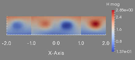
Magnetic field magnitude in the plane plane y=0.
|
 1.8.5
1.8.5 
