Introduction

In this example, we check the correctness of the module for interpolation on a thermohydrodynamic problem. The simulation is the next part of test 31 ( $1$-periodic in $z$ manufactured solution). Between test 31 and 32, the mesh is changed and so is the number of processors in the meridian section (1 proc. to 5 proc.). An interpolation step takes place during the debug.

The domain of computation is $\Omega= \{ (r,\theta,z) \in {R}^3 : (r,\theta,z) \in (0,1) \times [0,2\pi) \times (0,1)\} $. We note $\Gamma= \partial \Omega$. It is composed of a solid and a fluid subdomain:

\begin{align*} \overline{\Omega} = \overline{\Omega_s} \cup \overline{\Omega_f}.\\ \end{align*}

The subdomains are defined followingly: $\Omega_s = \{ (r,\theta,z) \in {R}^3 : (r,\theta,z) \in (0,1/2) \times [0,2\pi) \times (0,1)\} $ and $\Omega_f= \{ (r,\theta,z) \in {R}^3 : (r,\theta,z) \in (1/2,1) \times [0,2\pi) \times (0,1)\} $. We note $\Gamma_f = \partial \Omega_f$.

We solve the temperature equations:

\begin{align*} \begin{cases} \partial_t T+ \tilde{\bu} \cdot \GRAD T - \DIV (\kappa \GRAD T) &= f_T, \\ T_{|\Gamma} &= T_\text{bdy} , \\ T_{|t=0} &= T_0, \end{cases} \end{align*}

in the domain $\Omega$. The extended velocity is defined by $\tilde{\bu} = \bu$ in $\Omega_f$ and $0$ in $\Omega_s$. The diffusivity is a piecewise constant function of space: $\kappa = \kappa_f$ in $\Omega_f$ and $\kappa_s$ in $\Omega_s$, with $\kappa_s = 10 \kappa_f$.

We solve the Navier-Stokes equations:

\begin{align*} \begin{cases} \partial_t\bu+\left(\ROT\bu\right)\CROSS\bu - \frac{1}{\Re}\LAP \bu +\GRAD p &= \alpha T \textbf{e}_z + \bef, \\ \DIV \bu &= 0, \\ \bu_{|\Gamma_f} &= \bu_{\text{bdy}} , \\ \bu_{|t=0} &= \bu_0, \\ p_{|t=0} &= p_0, \end{cases} \end{align*}

in the domain $\Omega_f$. We denote by $\textbf{e}_z$ the unit vector in the vertical direction.

The data are the source terms $f_T$ and $\bef$, the boundary data $T_\text{bdy}$ and $\bu_{\text{bdy}}$, the initial data $T_0$, $\bu_0$ and $p_0$. The parameters are the thermal diffusivities $\kappa_s$ and $\kappa_f$, the kinetic Reynolds number $\Re$ and the thermal gravity number $\alpha$. We recall that these parameters are dimensionless.

Manufactured solutions

We approximate the following analytical solutions:

\begin{align*} T(r,\theta,z,t) & = r^2(r-r_0)^2\sin(2\pi z)(1+\cos(\theta))\cos(t), \\ u_r(r,\theta,z,t) &= -2\pi (r-r_0)^2\cos(2\pi z)(1+\cos(\theta))\cos(t), \\ u_{\theta}(r,\theta,z,t) &= 2\pi (r-r_0)^2\cos(2\pi z)(1+\cos(\theta))\cos(t), \\ u_z(r,\theta,z,t) &= \frac{r-r_0}{r} \sin(2\pi z) ((3r-r_0)(1+\cos(\theta))+(r-r_0)\sin(\theta))\cos(t), \\ p(r,\theta,z,t) &= r^3 \sin(2\pi z) \cos(\theta) \cos(t), \end{align*}

where $r_0 = 1/2$ is the limit between solid and fluid regions. The velocity is the curl of a vector field, it is thus divergence free. As mentioned, the solution is $1$-periodic in $z$.

The source terms $f_T, \bef$ and the boundary datas $T_\text{bdy}, \bu_{\text{bdy}}$ are computed accordingly.

Generation of the mesh

The finite element mesh used for this test is named SOLID_FLUID_20.FEM and has a mesh size of $0.05$ for the P1 approximation. You can generate this mesh with the files in the following directory: ($SFEMaNS_MESH_GEN_DIR)/EXAMPLES/EXAMPLES_MANUFACTURED_SOLUTIONS/SOLID_FLUID_20. The following image shows the mesh for P1 finite elements.

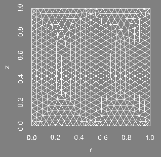
Finite element mesh (P1).

Information on the file `condlim.f90`

The initial conditions, boundary conditions and the forcing terms $\textbf{f}$ in the Navier-Stokes equations and $f_T$ in the temperature equations are set in the file condlim_test_32.f90, which is identical to condlim_test_31.f90. Here is a description of the subroutines and functions of interest.

The subroutine init_velocity_pressure initializes the velocity field and the pressure at the times $-dt$ and $0$ with $dt$ being the time step. This is done by using the functions vv_exact and pp_exact as follows:
time = 0.d0

DO i= 1, SIZE(list_mode)

mode = list_mode(i)

DO j = 1, 6

!===velocity

un_m1(:,j,i) = vv_exact(j,mesh_f%rr,mode,time-dt)

un (:,j,i) = vv_exact(j,mesh_f%rr,mode,time)

END DO

DO j = 1, 2

!===pressure

pn_m2(:) = pp_exact(j,mesh_c%rr,mode,time-2*dt)

pn_m1 (:,j,i) = pp_exact(j,mesh_c%rr,mode,time-dt)

pn (:,j,i) = pp_exact(j,mesh_c%rr,mode,time)

phin_m1(:,j,i) = pn_m1(:,j,i) - pn_m2(:)

phin (:,j,i) = Pn (:,j,i) - pn_m1(:,j,i)

ENDDO

ENDDO
The subroutine init_temperature initializes the temperature at the times $-dt$ and $0$ with $dt$ the time step. This is done by using the function temperature_exact as follows:
time = 0.d0

DO i= 1, SIZE(list_mode)

mode = list_mode(i)

DO j = 1, 2

tempn_m1(:,j,i) = temperature_exact(j, mesh%rr, mode, time-dt)

tempn (:,j,i) = temperature_exact(j, mesh%rr, mode, time)

ENDDO

ENDDO
The function vv_exact contains the analytical velocity field. It is used to initialize the velocity field and to impose Dirichlet boundary conditions on the velocity field.
1. The limit between fluid and solid region is defined:
  REAL(KIND=8) :: r0 = 0.5d0
2. The pi parameter is defined (as in each following subroutine).
  REAL(KIND=8) :: pi = 3.1415926535897932d0
3. We construct the radial and vertical coordinates r, z.
  r = rr(1,:)
  
  z = rr(2,:)
4. We define the velocity field depending of its TYPE (1 and 2 for the component radial cosine and sine, 3 and 4 for the component azimuthal cosine and sine, 5 and 6 for the component vertical cosine and sine) and of its mode m as follows:
  IF (TYPE==1) THEN
  
  IF ((m==0).OR.(m==1)) THEN
  
  vv = -2*pi*(r-r0)**2*cos(t)*cos(2*pi*z)
  
  ELSE
  
  vv = 0.d0
  
  END IF
  
  ELSE IF (TYPE==3) THEN
  
  IF ((m==0).OR.(m==1)) THEN
  
  vv = 2*pi*(r-r0)**2*cos(t)*cos(2*pi*z)
  
  ELSE
  
  vv = 0.d0
  
  END IF
  
  ELSE IF (TYPE==5) THEN
  
  IF ((m==0).OR.(m==1)) THEN
  
  vv = (r-r0)*cos(t)*sin(2*pi*z)/r * (3*r-r0)
  
  ELSE
  
  vv = 0.d0
  
  END IF
  
  ELSE IF (TYPE==6) THEN
  
  IF (m==1) THEN
  
  vv = (r-r0)*cos(t)*sin(2*pi*z)/r * (r-r0)
  
  ELSE
  
  vv = 0.d0
  
  END IF
  
  ELSE
  
  vv = 0.d0
  
  END IF
  
  where $t$ is the time. It is important to specify the null types or modes to avoid nonsense results.
The function pp_exact contains the analytical pressure.
1. We construct the radial and vertical coordinates r, z.
  r = rr(1,:)
  
  z = rr(2,:)
2. The pressure is non null only on the cosine compound and for the first mode.
  IF ((TYPE==1).AND.(m==1)) THEN
  
  vv = r**3*sin(2*pi*z)*cos(t)
  
  ELSE
  
  vv = 0.d0
  
  END IF
The function temperature_exact contains the analytical temperature. It is used to initialize the temperature and to impose Dirichlet boundary condition on the temperature.
1. The limit between fluid and solid region is defined:
  REAL(KIND=8) :: r0 = 0.5d0
2. We construct the radial and vertical coordinates r, z.
  r = rr(1,:)
  
  z = rr(2,:)
3. We define the temperature depending on its TYPE (1 and 2 for cosine and sine) and on its mode as follows:
  IF ((TYPE==1).AND.((m==0).OR.(m==1))) THEN
  
  vv = r**2*(r-r0)**2*sin(2*pi*z)*cos(t)
  
  ELSE
  
  vv = 0.d0
  
  END IF
The function source_in_temperature computes the source term $f_T$ of the temperature equations.
1. An array kappa for the value of the diffusivity at each node must be declared.
  REAL(KIND=8), DIMENSION(SIZE(rr,2)) :: vv, r, z, kappa
2. The limit between fluid and solid region is defined:
  REAL(KIND=8) :: r0 = 0.5d0
3. We construct the radial and vertical coordinates r, z.
  r = rr(1,:)
  
  z = rr(2,:)
4. The kappa array is filled based on the data file. The solid diffusivity is used for the region $r \le r_0$ and the fluid diffusivity is used in the fluid region $r > r_0$.
  DO i=1,SIZE(rr,2)
  
  IF (r(i).LE.r0) THEN
  
  kappa(i) = inputs%temperature_diffusivity(1)
  
  ELSE
  
  kappa(i) = inputs%temperature_diffusivity(2)
  
  END IF
  
  END DO
5. The source term $ f_T = \partial_t T+ \tilde{\bu} \cdot \GRAD T - \kappa \LAP T $ is defined in two parts. Firstly, we define the part $ \partial_t T - \kappa \LAP T $:
  IF (TYPE==1) THEN
  
  IF (m==0) THEN
  
  vv = - (-2*((2*pi**2*r**4 + 9*r*r0 - 4*pi**2*r**3*r0 - 2*r0**2 + 2*r**2*(-4.d0 + pi**2*r0**2))*kappa*Cos(t)) &
  
  + r**2*(r - r0)**2*Sin(t))*Sin(2*pi*z)
  
  ELSE IF (m==1) THEN
  
  vv = -(-((4*pi**2*r**4 + 16*r*r0 - 8*pi**2*r**3*r0 - 3*r0**2 + r**2*(-15.d0 + 4*pi**2*r0**2))*kappa*Cos(t)) &
  
  + r**2*(r - r0)**2*Sin(t))*Sin(2*pi*z)
  
  ELSE
  
  vv = 0.d0
  
  END IF
  
  ELSE
  
  vv = 0.d0
  
  END IF
  
  Secondly, we add the part $ \tilde{\bu} \cdot \GRAD T $, which is different from 0 only in the fluid:
  IF (TYPE==1) THEN
  
  IF (m==0) THEN
  
  DO i=1,size(rr,2)
  
  IF (r(i)>r0) THEN
  
  vv(i) = vv(i) + (-3*pi*r(i)*(r(i) - r0)**4*Cos(t)**2*Sin(4*pi*z(i)))/2.d0
  
  END IF
  
  END DO
  
  ELSE IF (m==1) THEN
  
  DO i=1,size(rr,2)
  
  IF (r(i)>r0) THEN
  
  vv(i) = vv(i) - 2*pi*r(i)*(r(i) - r0)**4*Cos(t)**2*Sin(4*pi*z(i))
  
  END IF
  
  END DO
  
  ELSE IF (m==2) THEN
  
  DO i=1,size(rr,2)
  
  IF (r(i)>r0) THEN
  
  vv(i) = vv(i) - 0.5*pi*(r(i)*(r(i) - r0)**4*Cos(t)**2*Sin(4*pi*z(i)))
  
  END IF
  
  END DO
  
  END IF
  
  END IF
  
  In the second part, the array is filled cell by cell because we have to test if the node is in the fluid region.
The function source_in_NS_momentum computes the source term $\alpha T \textbf{e}_z+\bef$ of the Navier-Stokes equations.
1. The coefficient $\alpha$ of the Boussinesq force is declared and the limit between fluid and solid region is defined:
  REAL(KIND=8) :: alpha, r0 = 0.5d0
2. The coefficient $\alpha$ is defined based on the data file.
  alpha = inputs%gravity_coefficient
3. We construct the radial and vertical coordinates r, z.
  r = rr(1,:)
  
  z = rr(2,:)
4. We construct the first part of the source term containing the Boussinesq force $\alpha T \be_z$ and the piece of $\bef$ that cancels it.
  IF (TYPE==5) THEN
  
  vv = alpha*(opt_tempn(:,1,i) - temperature_exact(1,rr,mode,time))
  
  ELSE IF (TYPE==6) THEN
  
  vv = alpha*(opt_tempn(:,2,i) - temperature_exact(2,rr,mode,time))
  
  ELSE
  
  vv = 0.d0
  
  END IF
  
  The array opt_temp is an input argument and produces the Boussinesq force. The temperature_exact function is defined in the same file and leads to the cancelling term of $\bef$.
5. The rest of the source term $ \partial_t\bu+\left(\ROT\bu\right)\CROSS\bu - \frac{1}{\Re}\LAP \bu +\GRAD p $ is then added. It depends on the TYPE (1-6) and the mode (0-2).

All the other subroutines present in the file condlim_test_32.f90 are not used in this test. We refer to the section Fortran file condlim.f90 for a description of all the subroutines of the condlim file.

Setting in the interpolation data file

We describe the interpolation data file needed to interpolate the fields of velocity, pressure and temperature at the end of test 31 on the new mesh. It is called debug_data_test_31_interpol and can be found in the directory ($SFEMaNS_DIR)/MHD_DATA_TEST_CONV_PETSC.

We indicate informations about the input simulation.
1. We indicate the number of processors in the meridian section.
  ===Number of processors in meridian section (Input)
  
  1
2. We indicate the problem type and wether there is a temperature field.
  ===Problem type (Input): (nst, mxw, mhd, fhd)
  
  'nst'
  
  ===Is there an input temperature field?
  
  .t.
3. We indicate the mesh informations.
  ===Directory and name of input mesh file
  
  '.' 'SOLID_FLUID_10.FEM'
  
  ===Is input mesh file formatted (true/false)?
  
  .t.
We indicate informations about the output simulation.
1. We indicate the number of processors in the meridian section.
  ===Number of processors in meridian section (Output)
  
  5
2. We indicate the problem type and wether there is a temperature field.
  ===Problem type (Output): (nst, mxw, mhd, fhd)
  
  'nst'
  
  ===Is there an output temperature field?
  
  .t.
3. We indicate the mesh informations.
  ===Directory and name of input mesh file
  
  '.' 'SOLID_FLUID_20.FEM'
  
  ===Is input mesh file formatted (true/false)?
  
  .t.
We detail the process of interpolation.
1. We indicate wether the mesh changes.
  ===Should data be interpolated on new mesh? (True/False)
  
  .t.
  
  It could not be the case if the user only wanted to change the number of processors in the meridian section. The module for mesh interpolation must be used in this case too.
2. We indicate the number of time steps we want to interpolate. We are only interested in the last time step here.
  ===How many files (times steps) should be converted?
  
  1
3. We set the starting index. Restart files are indexed with a number. We have written only one restart file (for each field). We select 1.
  ===What is the starting index? (suite*_I*index.mesh*), index is an integer in [1,999]
  
  1
4. We indicate the number of Fourier modes.
  ===Number of Fourier modes
  
  3
We set the periodic boundaries (for output simulation).
1. We indicate the number of couples of periodic interfaces. In our case, there is only one, the couple of interfaces 4 (bottom) and 2 (top)
  ===How many pieces of periodic boundary?
  
  1
  
  There could have been a second couple if we had given a different number to the top (and bottom) boundaries of solid and fluid subdomains.
2. We indicate the interfaces of each couple, and the coordinates in the plan $(r,z)$ of the vector that joins them. The vector that joins interfaces 4 and 2 is the vector $\be_z$.
  ===Indices of periodic boundaries and corresponding vectors
  
  4 2 0.d0 1.d0
  
  If there was additional couples, corresponding lines should be written below.
We set the number of domains and their label, see the files associated to the generation of the mesh, where the code approximates the Navier-Stokes equations (for output simulation).
===Number of subdomains in Navier-Stokes mesh

1

===List of subdomains for Navier-Stokes mesh

2
We set the number of domains and their label, see the files associated to the generation of the mesh, where the code approximates the temperature equation (for output simulation).
===Number of subdomains in temperature mesh

2

===List of subdomains for temperature mesh

1 2
We set the interfaces between regions where only the temperature is solved and regions where velocity and tenperature is solved (for output simulation). It is necessary to impose boundary conditions on the velocity at these interfaces.
===Number of interfaces between velocity and temperature only domains (for nst applications)

1

===List of interfaces between velocity and temperature only domains (for nst applications)

3

Setting in the data file

We describe the data file of this test. It is called debug_data_test_32 and can be found in the directory ($SFEMaNS_DIR)/MHD_DATA_TEST_CONV_PETSC.

We use a formatted mesh by setting:
===Is mesh file formatted (true/false)?

.t.
The path and the name of the mesh are specified with the two following lines:
===Directory and name of mesh file

'.' 'SOLID_FLUID_20.FEM'

where '.' refers to the directory where the data file is, meaning ($SFEMaNS_DIR)/MHD_DATA_TEST_CONV_PETSC.
We use five processors in the meridian section.
===Number of processors in meridian section

5
We solved the problem for $3$ Fourier modes.
===Number of Fourier modes

3

The Fourier modes are not detailed so the first three modes $0,1,2$ are solved.
We use $3$ processors in Fourier space.
===Number of processors in Fourier space

1

It means that each processors is solving the problem for the $3$ Fourier modes.
We approximate the Navier-Stokes equations by setting:
===Problem type: (nst, mxw, mhd, fhd)

'nst'
We restart the computations from previous results.
===Restart on velocity (true/false)

.t.

===Restart on temperature (true/false)

.t.

The computation starts from the time $t=1$ (end of test 31).
We use a time step of $0.005$ and solve the problem over $200$ time iterations.
===Time step and number of time iterations

5.d-3 200
We read the metis partition provided by the mesh interpolation module.
===Do we read metis partition? (true/false)

.t.
We set the periodic boundaries.
1. We indicate the number of couples of periodic interfaces. In our case, there is only one, the couple of interfaces 4 (bottom) and 2 (top)
  ===How many pieces of periodic boundary?
  
  1
  
  There could have been a second couple if we had given a different number to the top (and bottom) boundaries of solid and fluid subdomains.
2. We indicate the interfaces of each couple, and the coordinates in the plan $(r,z)$ of the vector that joins them. The vector that joins interfaces 4 and 2 is the vector $\be_z$.
  ===Indices of periodic boundaries and corresponding vectors
  
  4 2 0.d0 1.d0
  
  If there was additional couples, corresponding lines should be written below.
We set the number of domains and their label, see the files associated to the generation of the mesh, where the code approximates the Navier-Stokes equations.
===Number of subdomains in Navier-Stokes mesh

1

===List of subdomains for Navier-Stokes mesh

2
We set the number of boundaries with Dirichlet conditions on the velocity field and give their respective labels.
===How many boundary pieces for full Dirichlet BCs on velocity?

2

===List of boundary pieces for full Dirichlet BCs on velocity

3 5
We set the kinetic Reynolds number $\Re$.
===Reynolds number

1.d0
We give information on how to solve the matrix associated to the time marching of the velocity.
1. ===Maximum number of iterations for velocity solver
  
  100
2. ===Relative tolerance for velocity solver
  
  1.d-6
  
  ===Absolute tolerance for velocity solver
  
  1.d-10
3. ===Solver type for velocity (FGMRES, CG, ...)
  
  GMRES
  
  ===Preconditionner type for velocity solver (HYPRE, JACOBI, MUMPS...)
  
  MUMPS
We give information on how to solve the matrix associated to the time marching of the pressure.
1. ===Maximum number of iterations for pressure solver
  
  100
2. ===Relative tolerance for pressure solver
  
  1.d-6
  
  ===Absolute tolerance for pressure solver
  
  1.d-10
3. ===Solver type for pressure (FGMRES, CG, ...)
  
  GMRES
  
  ===Preconditionner type for pressure solver (HYPRE, JACOBI, MUMPS...)
  
  MUMPS
We give information on how to solve the mass matrix.
1. ===Maximum number of iterations for mass matrix solver
  
  100
2. ===Relative tolerance for mass matrix solver
  
  1.d-6
  
  ===Absolute tolerance for mass matrix solver
  
  1.d-10
3. ===Solver type for mass matrix (FGMRES, CG, ...)
  
  CG
  
  ===Preconditionner type for mass matrix solver (HYPRE, JACOBI, MUMPS...)
  
  MUMPS
We solve the temperature equation.
===Is there a temperature field?

.t.
We set the coefficient $\alpha$ of Boussinesq force.
===Non-dimensional gravity coefficient

1.d0
We set the number of domains and their label, see the files associated to the generation of the mesh, where the code approximates the temperature equation.
===Number of subdomains in temperature mesh

2

===List of subdomains for temperature mesh

1 2
We set the thermal diffusivity $\kappa$.
===Diffusivity coefficient for temperature (1:nb_dom_temp)

10.d0 1.d0
We set the number of boundaries with Dirichlet conditions on the velocity and give their respective labels.
===How many boundary pieces for Dirichlet BCs on temperature?

1

===List of boundary pieces for Dirichlet BCs on temperature

5
We set the interfaces between regions where only the temperature is solved and regions where velocity and temperature is solved. It is necessary to impose boundary conditions on the velocity at these interfaces.
===Number of interfaces between velocity and temperature only domains (for nst applications)

1

===List of interfaces between velocity and temperature only domains (for nst applications)

3
We give information on how to solve the matrix associated to the time marching of the temperature.
1. ===Maximum number of iterations for temperature solver
  
  100
2. ===Relative tolerance for temperature solver
  
  1.d-6
  
  ===Absolute tolerance for temperature solver
  
  1.d-10
3. ===Solver type for temperature (FGMRES, CG, ...)
  
  GMRES
  
  ===Preconditionner type for temperature solver (HYPRE, JACOBI, MUMPS...)
  
  MUMPS
To get the total elapse time and the average time in loop minus initialization, we write:
===Verbose timing? (true/false)

.t.

These informations are written in the file lis when you run the shell debug_SFEMaNS_template.

Outputs and value of reference

The outputs of this test are computed with the file post_processing_debug.f90 that can be found in: ($SFEMaNS_DIR)/MHD_DATA_TEST_CONV_PETSC.

To check the well behavior of the code, we compute four quantities:

The L2-norm of error on u divided by the L2-norm of u exact.
The L2-norm of error on p divided by L2-norm of p exact.
The L2-norm of error on T divided by L2-norm of T exact.
The H1-norm of error on T divided by H1-norm of T exact.

These quantities are computed at the final time $t=1$. They are compared to reference values to attest of the correct behavior of the code. These values of reference are in the last lines of the file debug_data_test_32 in ($SFEMaNS_DIR)/MHD_DATA_TEST_CONV_PETSC. They are equal to:

============================================
(SOLID_FLUID_20.FEM)
===Reference results
6.06639948859780695E-005  L2-norm of error on u / L2-norm of u exact
7.38878983488354922E-003  L2-norm of error on p / L2-norm of p exact
2.45969800747957744E-005  L2-norm of error on T / L2-norm of T exact
2.77731794127341280E-004  H1-norm of error on T / H1-norm of T exact

To conclude this test, we display the profile of the approximated, pressure, velocity magnitude and temperature at the final time. These figures are done in the plane $y=0$ which is the union of the half plane $\theta=0$ and $\theta=\pi$.

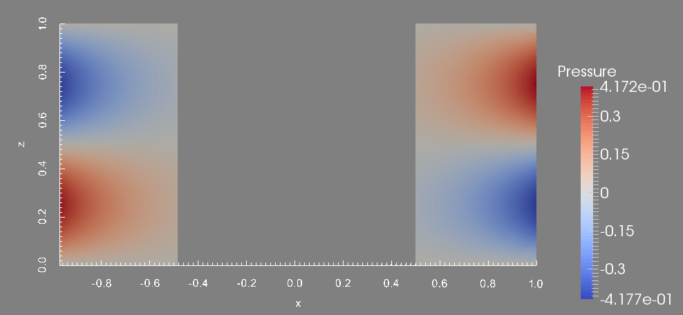
Pressure in the plane plane y=0.

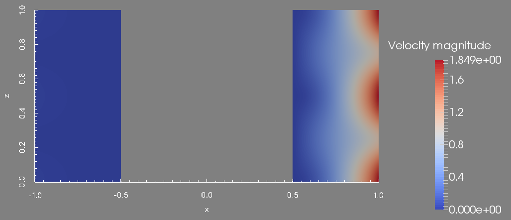
Velocity magnitude in the plane y=0.

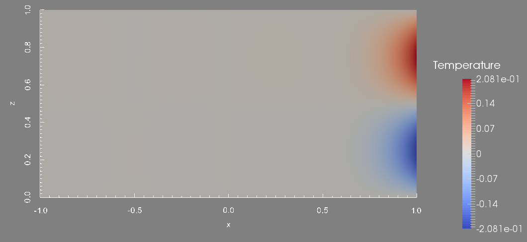
Temperature in the plane y=0.